The Granger causality tests if one variable “Granger causes” another variable and vice versa, using restricted autoregressive lags and unrestricted distributive lag models. Typically, predictive causality in finance and economics is tested by measuring the ability to predict the future values of a time series using prior values of another time series. A simpler definition might be that a time-series variable A can Granger cause another time-series variable B if predictions of the value of B based solely on its own prior values and on the prior values of A are comparatively better than predictions of B based solely on its own past values. For example, Figure 9.49 illustrates two time-series variables, A and B. The two null hypotheses tested are that there is no Granger causality of A on B and also between B and A. We see that the p-values for both directions are greater than an alpha of 0.05, so we cannot reject the null hypothesis and conclude that neither A Granger causes B nor B Granger causes A, when both are lagged for 3 periods (this is the value 3 in the input box).
The Granger causality model can only be run pairwise and assumes that the time-series variable is stationary or not stochastic. If a time-series is suspected to have nonstationary effects, we can run the Augmented Dickey–Fuller test (see Figure 9.50), where the null hypothesis is that the series is nonstationary, has a unit root, or I(1) process, and is potentially stochastic. The example BizStats results indicate that the variable is stationary (the null hypothesis is rejected with a p-value of 0.0442).
However, if a time-series variable is nonstationary and stochastic, you can still attempt to forecast this series in several ways:
- Compute the difference to potentially make the series stationary. For example, stock prices are nonstationary and stochastic, whereas its difference, i.e., the calculated stock returns, tend to be stationary and more predictable than the raw stock prices.
- Run a stochastic process model, for example, a geometric Brownian motion random walk process, mean-reversion process, jump-diffusion process, or other mixed processes. These are typically used to forecast stock prices for the purposes of modeling and valuing stock options, real options, and employee stock options. Both Risk Simulator (see Chapter 11’s stochastic forecasting section) and BizStats (Figure 9.51) support these methods.
- If there is another nonstationary variable, you can test if these two series are cointegrated. For example, you can use the Engle–GrangerError Correction Model assuming the variables exhibit cointegration. If two time-series variables are nonstationary in the first order, I(1), as tested using the Augmented Dickey–Fuller test, and when both variables are cointegrated, the error correction model can be used for estimating short-term and long-term effects of one time-series on the another. The error correction comes from previous periods’ deviation from a long-run equilibrium, where the error influences its short-run dynamics (Figure 9.52).
- Apply a data filter to smooth out the disturbances such as the Hodrick–Prescott filter (Figure 9.53). This filter allows you to remove the cyclical effects of raw time-series data. The filter helps generate a smoothed curve of a time-series variable that is sensitive to longer-term fluctuations rather than short-term impacts. The key is to choose the correct smoothing parameter, which can sometimes require trial and error.
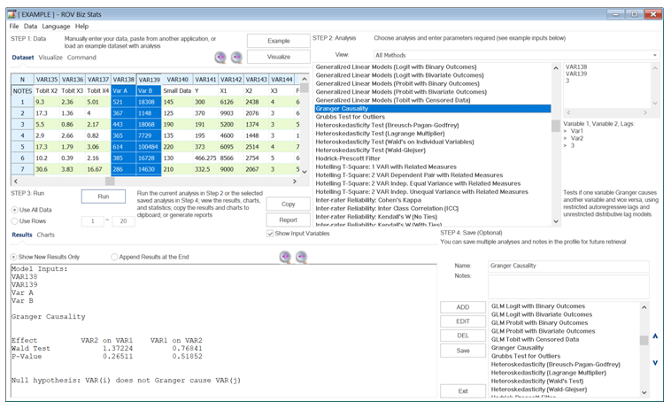
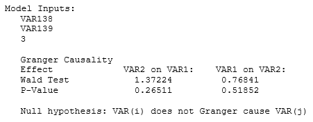
Figure 9.49: Granger Causality
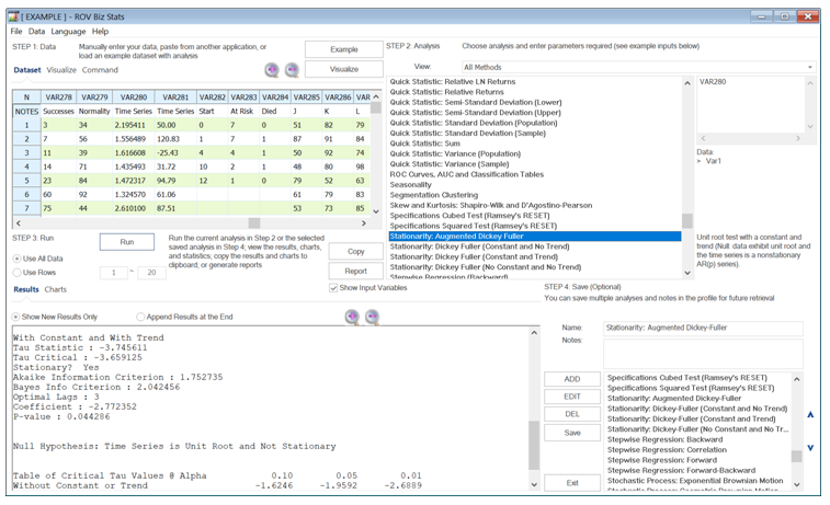
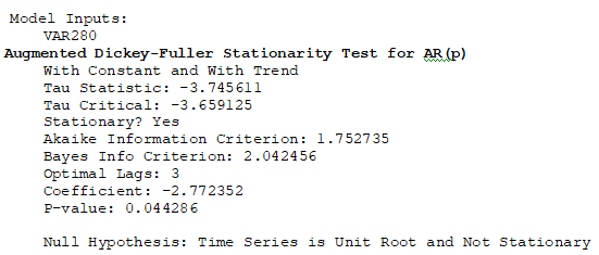
Figure 9.50: Augmented Dickey–Fuller Test for Stationarity
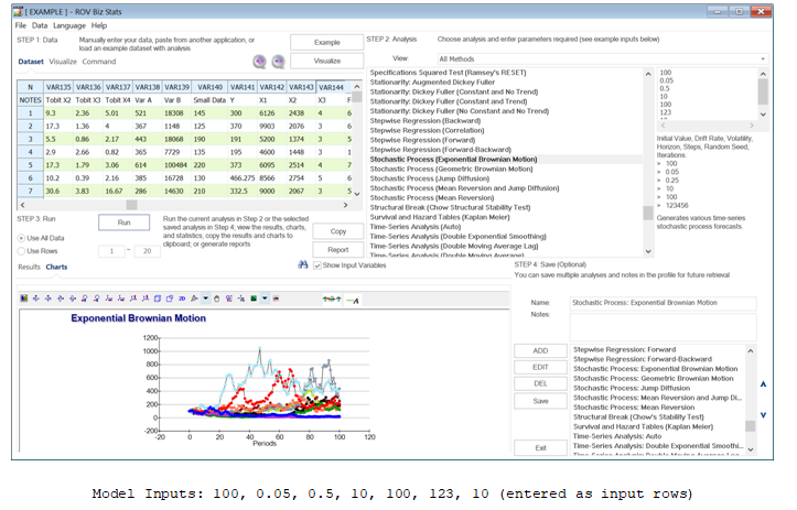
Figure 9.51: Stochastic Processes
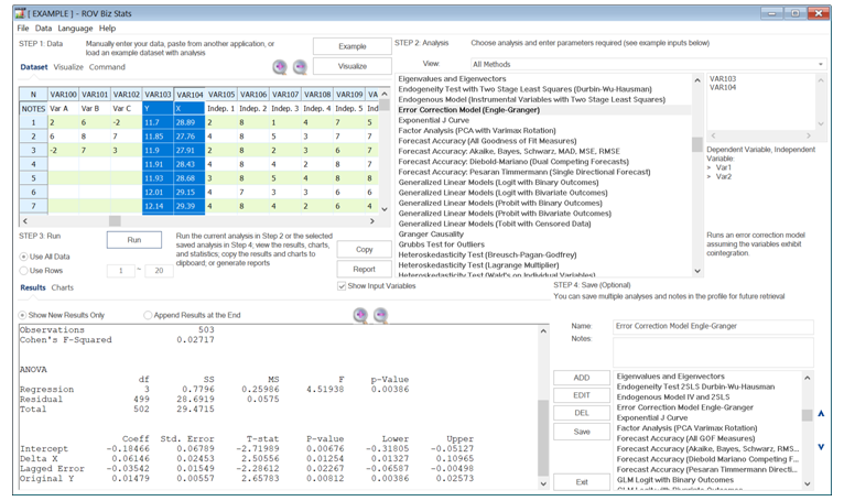
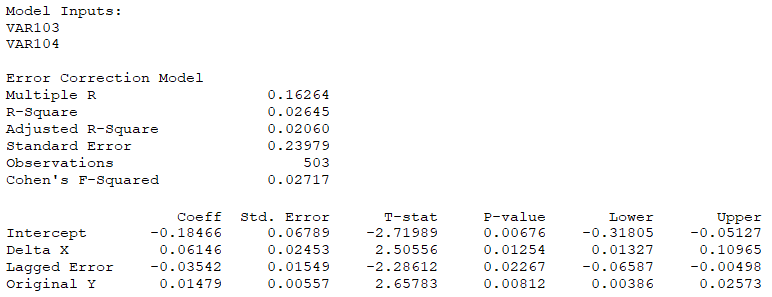
Figure 9.52: Error Correction Model
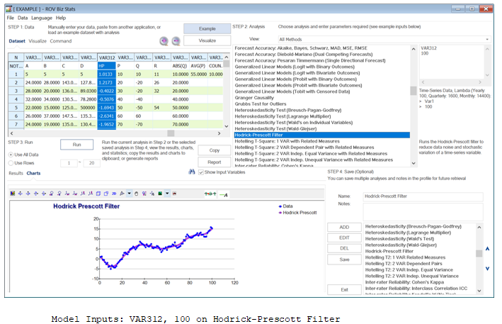
Figure 9.53: Hodrick–Prescott Filtering