File Name: Optimization – Inventory Optimization
Location: Modeling Toolkit | Optimization | Inventory Optimization
Brief Description: Illustrates how to run an optimization on manufacturing inventory to maximize profits and minimize costs subject to manufacturing capacity constraints
Requirements: Modeling Toolkit, Risk Simulator
This model is used to find the optimal allocation of parts in a manufacturer’s portfolio of inventory. In the model, eight different parts are shown, with their respective prices per unit (Figure 96.1). The demand for these parts is divided into four phases or cycles. For example, in the automotive aftermarket, certain parts are required more or less at certain times in the car’s lifecycle (e.g., fewer parts may be needed during the first 3 years of a car’s life than perhaps in years 4 to6, or years 7 to10, versus over 10 years) or parts of a machine, or the inventory in a retail shop during the four seasons in a year, and so forth. The demand levels in these cycles for each part is simulated (assumptions have already been preset in the model) and can be based on expert opinions, expectations, forecasts, or historical data (e.g., using distributional fitting methods in Risk Simulator).
In this model, if the manufacturer makes a higher quantity of a product than it can sell, there will be an added holding cost per unit (storage cost, opportunity cost, cost of money, etc.). Thus, it is less profitable to make too many units, but too few units mean lost sales. In other words, if the manufacturer makes too much, it loses money because it could have made some more of something else, but if it makes too little of a product, it should have made more to sell more of the product and make a profit. So an optimal inventory and manufacturing quantity is required. This model is used to find the best allocation of parts to manufacture given the uncertainty in demand and, at the same time, to maximize profits while minimizing cost.
However, the manufacturer has constraints. It cannot manufacture too many units of a single part due to resource, budget, and manufacturing constraints (size of the factory, cycle time, manufacturing time, cost considerations, etc.). For example, say the firm cannot produce more than 100,000 units per part, and during each manufacturing or seasonal cycle, it cannot produce more than 250,000 units, and the total parts produced are set at no more than 800,000 units. In short, the problem can be summarized as:
- Objective: Maximize total net revenues
- Problem: Find the best allocation of parts to maximize net revenues
(surplus and shortages are expensive) - Constraints: Each part cannot exceed 100,000 units
Each cycle cannot exceed 250,000 units
Each part in each cycle is between 15,000 and 35,000 units
Total parts cannot exceed 800,000 units - Assumptions: Surplus units has a holding inventory cost of $1
One very simple allocation is to produce an equal amount (e.g., 25,000 units per part, per cycle, thereby hitting all the constraints) as illustrated in Figure 96.1. The total net revenue from such a simple allocation is found to be $105,082,000.
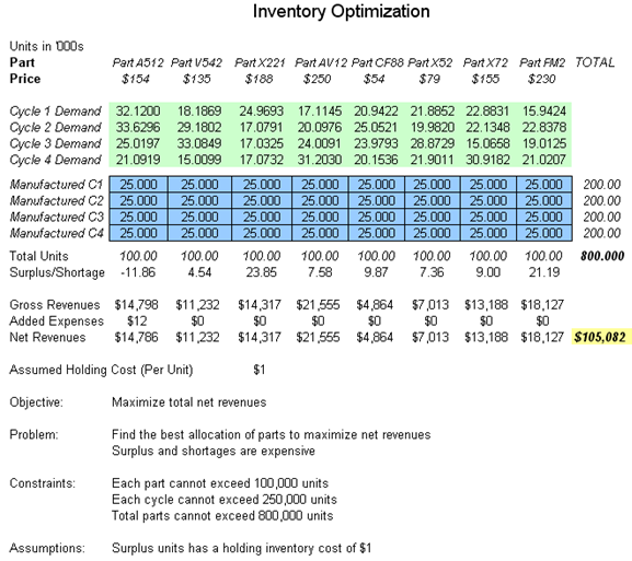
Figure 96.1: Inventory model before optimization
Optimization Procedure (Predefined)
In contrast, an optimization can be set up to solve this problem. The optimization has already been set up in the model and is ready to run. To run it:
- Go to the Optimization Model worksheet and click on Risk Simulator | Change Profile and select the Inventory Optimization profile.
- Click on the Run Optimization icon or click on Risk Simulator | Optimization | Run Optimization and click OK.
- Click Replace when optimization is completed. The results show the optimal allocation of manufactured parts that maximizes the total net profit, increasing it from $105.082 million to $110.116 million (Figure 96.2). Clearly, optimization has created value.
- Using these optimal allocations, run a simulation (the assumptions and forecasts have been predefined in the model) by clicking on the RUN icon or select Risk Simulator | Run Simulation.
- On the Net Revenues forecast chart, select Two-Tail and type in 90 in the Certainty box, and hit TAB on the keyboard to obtain the 90% confidence interval (between $105 million and $110 million). View the Statistics tab to obtain the mean expected value of $108 million for the net revenues.
- Select Right-Tail and type in 105082 in the Value box, to find the probability that this optimal allocation’s portfolio of manufactured products (Figure 96.2) will exceed the simple equal allocation’s net revenues seen in Figure 96.1. The results indicate that there is a 95.40% probability that by using this optimal portfolio, the manufacturer will make more net profits than going with a simple equal allocation (Figure 96.3).
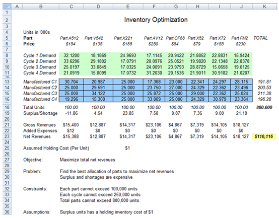
Figure 96.2: Optimized results
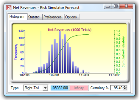
Figure 96.3: Optimized net revenues
Optimization Procedure (Manual)
To set up the model again from scratch, follow the instructions below:
- Go to the Optimization Model worksheet and click on Risk Simulator | New Profile and give the profile a new name. You may have to reset the decision variables to some starting value (i.e., make the cells C13:J16 all 25 as a starting point) so that you can immediately see when the optimization generates new values.
- Click on cell K23 and make it the objective to maximize (Risk Simulator | Optimization | Set Objective and select Maximize).
- Click on cell C13 and make it a decision variable (Risk Simulator | Optimization | Set Decision), and select Continuous for getting a continuous variable (we need this because the model’s values are in thousands of units and thousands of dollars) and set the bounds to be between 15 and 35 (you can set your own bounds but these are typically constraints set by the manufacturer) to signify that the manufacturer can make only between 15,000 and 35,000 units of this part per cycle due to resource and budget or machine constraints.
- Set the constraints by clicking on Risk Simulator | Optimization | Constraints and select ADD for adding a new constraint. Add the three additional constraints in the model, namely, cells K13 to K16 <= 250 for each cell, C18 to J18 <= 100 for each cell, and K18 <=800. Do this one constraint at a time (Figure 96.4). Put your own constraints as required.
- Click on the Run Optimization icon or click on Risk Simulator | Optimization | Run Optimization. Look through the tabs to make sure everything is set up correctly. Click on the Method tab and select Static Optimization and click OK to run the optimization.
- Click Replace when optimization is completed. The results illustrate that the optimal allocation of manufactured parts that maximizes net profit, increases it from $105.082 million to $110.116 million. Clearly, optimization has created value.
- Using these optimal allocations, run a simulation (the assumptions and forecasts have been predefined in the model) by clicking on the RUN icon or select Risk Simulator | Run Simulation.
- On the Net Revenues forecast chart, select Two-Tail and type in 90 in the Certainty box, and hit TAB on the keyboard to obtain the 90% confidence interval (between $105 million and $110 million). View the Statistics tab to obtain the mean expected value of $108 million for the net revenues.
- Select Right-Tail and type in 105082 in the Value box, to find the probability that this optimal allocation’s portfolio of manufactured products will exceed the simple equal allocation’s net revenues seen previously.
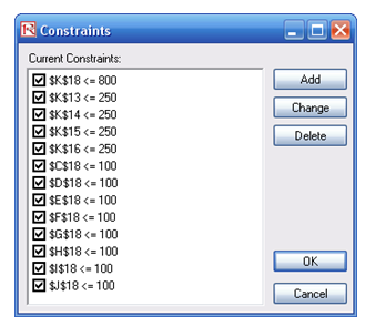
Figure 96.4: Setting constraints one at a time