File Name: Analytics – Statistical Analysis
Location: Modeling Toolkit | Analytics | Statistical Analysis
Brief Description: Applies the Statistical Analysis tool to determine the key statistical characteristics of your dataset, including linearity, nonlinearity, normality, distributional fit, distributional moments, forecastability, trends, and the stochastic nature of the data
Requirements: Modeling Toolkit, Risk Simulator
This model provides a sample dataset on which to run the Statistical Analysis tool in order to determine the statistical properties of the data. The diagnostics run includes checking the data for various statistical properties.
Procedure
To run the analysis, follow the instructions below:
- Go to the Data worksheet and select the data including the variable names (cells D5:F55).
- Click on Risk Simulator | Analytical Tools | Statistical Analysis (Figure 8.1).
- Check the data type: whether the data selected are from a single variable or multiple variables arranged in columns. In our example, we assume that the data areas selected are from multiple variables. Click OK when finished.
- Choose the statistical tests you wish performed. The suggestion (and by default) is to choose all the tests. Click OK when finished (Figure 8.2).
Spend some time going through the reports generated to get a better understanding of the statistical tests performed.
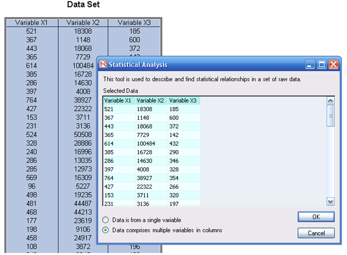
Figure 8.1: Running the Statistical Analysis tool
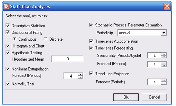
Figure 8.2: Statistical tests
The analysis reports include the following statistical results:
- Descriptive Statistics: Arithmetic and geometric mean, trimmed mean (statistical outliers are excluded in computing its mean value), standard error and its corresponding statistical confidence intervals for the mean, median (the 50th percentile value), mode (most frequently occurring value), range (maximum less minimum), standard deviation and variance of the sample and population, confidence interval for the population standard deviation, coefficient of variability (sample standard deviation divided by the mean), first and third quartiles (25th and 75th percentile value), skewness, and excess kurtosis.
- Distributional Fit: Fitting the data to all 24 discrete and continuous distributions in Risk Simulator to determine which theoretical distribution best fits the raw data and proving it with statistical goodness-of-fit results (Kolmogorov-Smirnov and Chi-Square tests’ p-value results).
- Hypothesis Tests: Single variable one-tail and two-tail tests to see if the raw data is statistically similar or different from a hypothesized mean value.
- Nonlinear Extrapolation: Tests for nonlinear time-series properties of the raw data, to determine if the data can be fitted to a nonlinear curve.
- Normality Test: Fits the data to a normal distribution using a theoretical fitting hypothesis test to see if the data is statistically close to a normal distribution.
- Stochastic Calibration: Using the raw data, various stochastic processes are fitted (Brownian motion, jump-diffusion, mean-reversion, and random walk processes) and the levels of fit as well as the input assumptions are automatically determined.
- Autocorrelation and Partial Autocorrelation: The raw dataset is tested to see if it is correlated to itself in the past by applying some econometric estimations and tests of autocorrelation and partial autocorrelation coefficients.
- Time-Series Forecasting: Eight most-commonly used time-series decomposition models are applied to determine if the raw dataset follows any trend and seasonality, and whether the time-series is predictable.
- Trend Analysis: A linear time-trend is tested to see if the data has any appreciable trend, using a linear regression approach.
Figure 8.3 shows a sample report generated by Risk Simulator that analyzes the statistical characteristics of your dataset, providing all the requisite distributional moments and statistics to help you determine the specifics of your data, including the skewness and extreme events (kurtosis and outliers). The descriptions of these statistics are listed in the report for your review. Each variable will have its own set of reports.
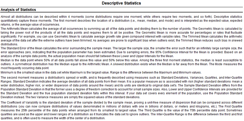
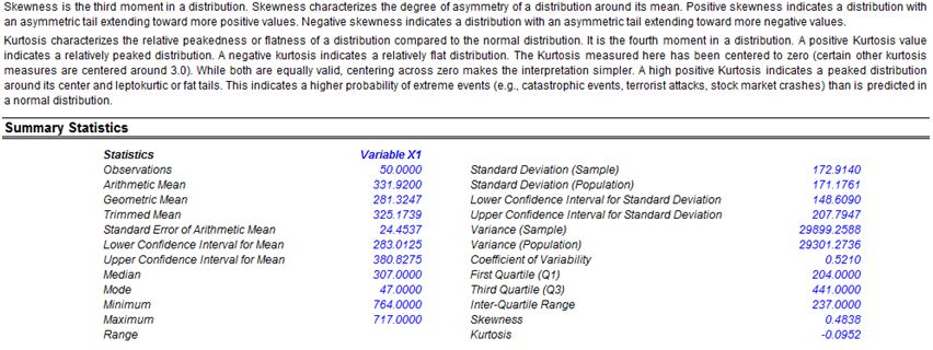
Figure 8.3: Sample report on descriptive statistics
Figure 8.4 shows the results of taking your existing dataset and creating a distributional fit on 24 distributions. The best-fitting distribution (after Risk Simulator goes through multiple iterations of internal optimization routines and statistical analyses) is shown in the report, including the test statistics and requisite p-values indicating the level of fit. For instance, Figure 8.4’s example dataset shows a 99.54% fit to a normal distribution with a mean of 319.58 and a standard deviation of 172.91. In addition, the actual statistics from your dataset are compared to the theoretical statistics of the fitted distribution, providing yet another layer of comparison. Using this methodology, you can take a large dataset and collapse it into a few simple distributional assumptions that can be simulated, thereby vastly reducing the complexity of your model or database while at the same time adding an added element of analytical prowess to your model by including risk analysis.
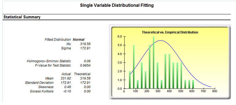
Figure 8.4: Sample report on distributional fitting
Sometimes, you might need to determine if the dataset’s statistics are significantly different than a specific value. For instance, if the mean of your dataset is 0.15, is this statistically significantly different than, say, zero? What about if the mean was 0.5 or 10.5? How far enough away does the mean have to be from this hypothesized population value to be deemed statistically significantly different? Figure 8.5 shows a sample report of such a hypothesis test.
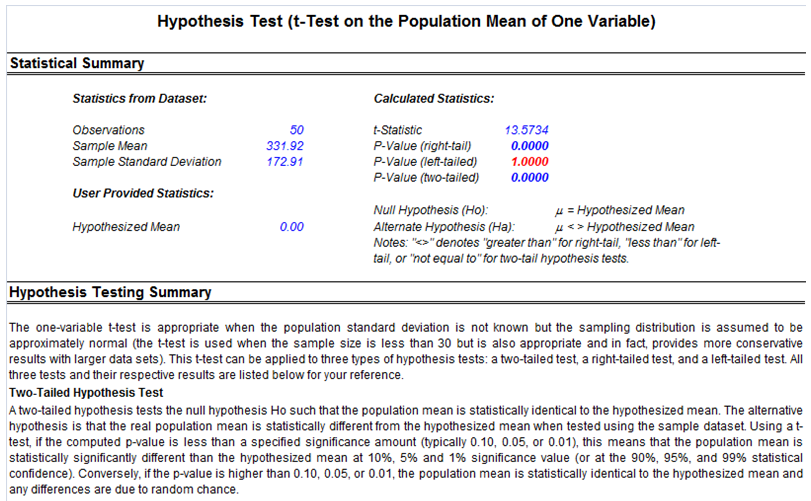
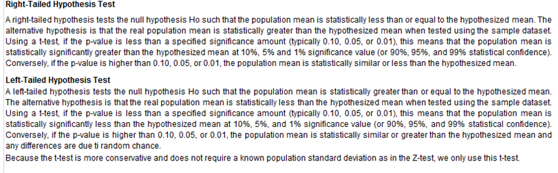
Figure 8.5: Sample report on theoretical hypothesis tests
Figure 8.6 shows the test for normality. In certain financial and business statistics, there is a heavy dependence on normality (e.g., asset distributions of option pricing models, normality of errors in a regression analysis, hypothesis tests using t-tests, Z-tests, analysis of variance, and so forth). This theoretical test for normality is automatically computed as part of the Statistical Analysis tool.
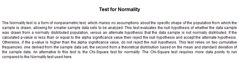
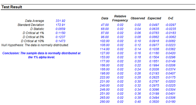
Figure 8.6: Sample report on testing for normality
If your dataset is a time-series variable (i.e., data that has an element of time attached to them, such as interest rates, inflation rates, revenues, and so forth, that are time-dependent) then the Risk Simulator data analysis reports shown in Figures 8.7 to 8.11 will help in identifying the characteristics of this time-series behavior, including the identification of nonlinearity (Figure 8.7) versus linear trends (Figure 8.8), or a combination of both where there might be some trend and nonlinear seasonality effects (Figure 8.9). Sometimes, a time-series variable may exhibit a relationship to the past (autocorrelation). The report shown in Figure 8.10 analyzes if these autocorrelations are significant and useful in future forecasts, that is, to see if the past can truly predict the future. Finally, Figure 8.11 illustrates the report on nonstationarity to test if the variable can or cannot be readily forecasted with conventional means (e.g., stock prices, interest rates, foreign exchange rates are very difficult to forecast with conventional approaches and require stochastic process simulations) and identifies the best-fitting stochastic models such as a Brownian motion random walk, mean-reversion and jump-diffusion processes, and provides the estimated input parameters for these forecast processes.
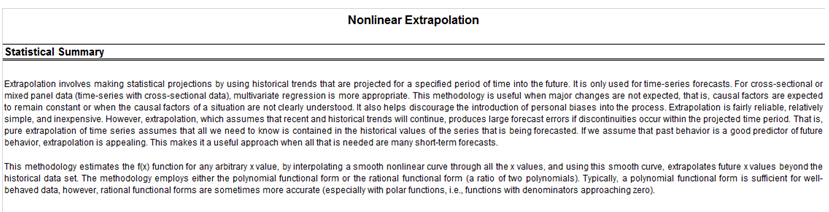
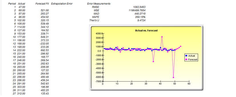
Figure 8.7: Sample report on nonlinear extrapolation forecast (nonlinear trend detection)
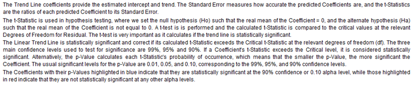
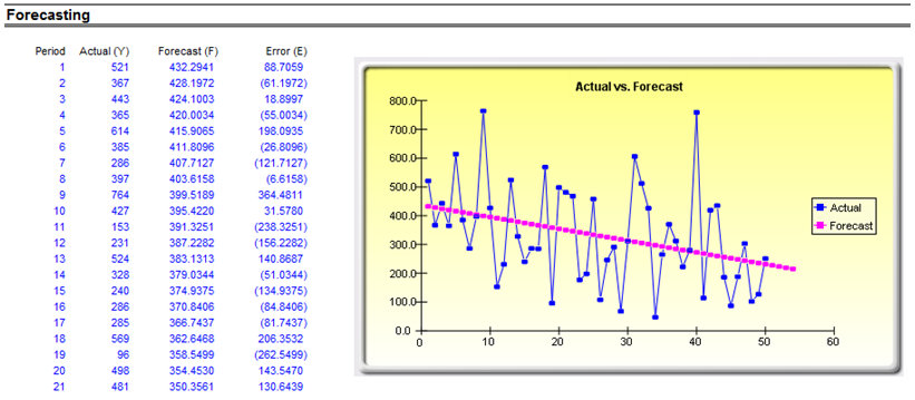
Figure 8.8: Sample report on trend-line forecasts (linear trend detection)
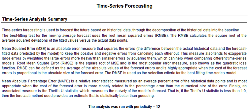
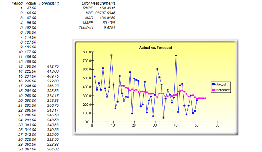
Figure 8.9: Sample report on time-series forecasting (seasonality and trend detection)
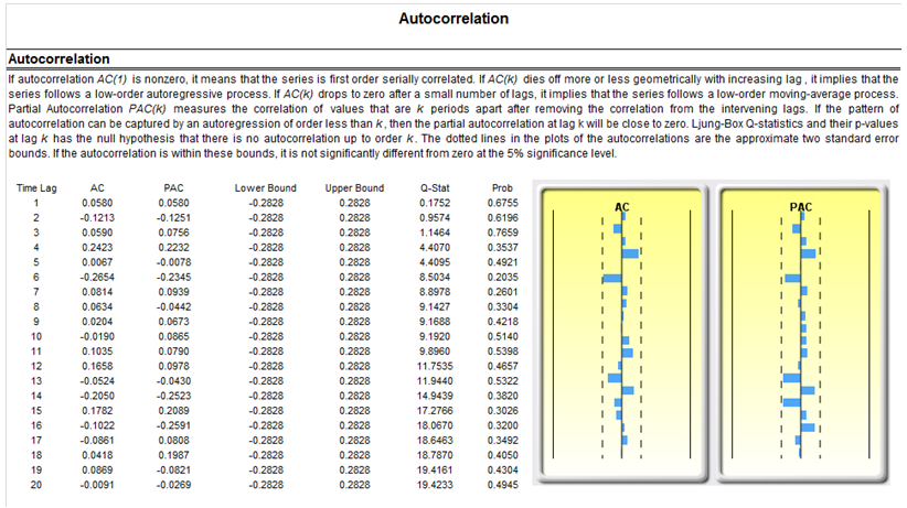
Figure 8.10: Sample report on autocorrelation (past relationship and correlation detection)
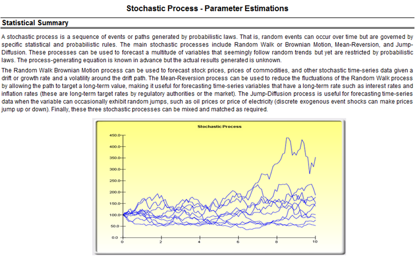
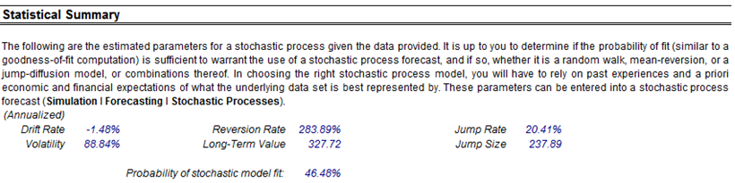
Figure 8.11: Sample report on stochastic parameter calibration (nonstationarity detection)