The case of operational risk is undoubtedly the most difficult to measure and model. The opposite of market risk, by its definition, operational risk data is not only scarce, but biased, unstable, and unchecked in the sense that the most relevant operational risk events do not come identified in the balance sheet of any financial institution. Since the modeling approach is still based on VaR logic, whereby the model utilizes past empirical data to project expected results, modeling operational risk is a very challenging task. As stated, market risk offers daily, publicly audited information to be used and modeled. Conversely, operational risk events are, in most cases, not public, not identified in the general ledger, and, in many instances, not identified at all. But the utmost difficulty comes from the proper definition of operational risk. Even if we managed to go about the impossible task of identifying each and every operational risk event, we would still have very incomplete information. The definition of operational risk entails events generated by failures in people, processes, systems, and external events. With market risk, asset prices can either go up or down, or stay unchanged. With operational risk, an unknown event that has never occurred before can take place in the analysis period and materially affect operations even without its being an extreme tail event.
So, the logic of utilizing similar approaches for such different information availability and behavior requires very careful definitions and assumptions. With this logic in mind, the Basel Committee has defined that in order to model operational risk properly, banks need to have four sources of operational risk data: internal losses, external losses, business environment and internal control factors, and stressed scenarios. Known as the four elements of operational risk, the Basel Committee recommends that they are taken into account when modeling. For smaller banks, and smaller countries, this recommendation poses a definitive challenge, because many times these elements are not developed enough, or not present at all. In this light, most banks have resorted to just using internal data to model operational risk. This approach comes with some shortcomings and more assumptions and should be taken as an initial step that considers the later development of the other elements as they become available. The example shown in Figure 5.1 looks at the modeling of internal losses as a simplified approach usually undertaken by smaller institutions. Since operational risk information is scarce and biased, it is necessary to “complete” the loss distributions with randomly generated data. The most common approach for the task is the use of Monte Carlo risk simulations (Figures 5.2, 5.3, and 5.4) that allow for the inclusion of more stable data and for the fitting of the distributions into predefined density functions.
Basel III and Basel IV regulations allow for the use of multiple approaches when it comes to computing capital charge on operational risk, defined by the Basel Committee as losses resulting from inadequate or failed internal processes, people, and systems or from external events, which includes legal risk, but excludes any strategic and reputational risks.
- Basic Indicator Approach (BIA) uses the positive Gross Income of the last 3 years applied to an Alpha multiplier.
- The Standardized Approach (TSA) uses the positive Gross Income of 8 distinct business lines with its own Betarisk-weighted coefficients.
- Alternate Standardized Approach (ASA) is based on the TSA method and uses Gross Income but applies Total Loans and Advances for the Retail and Commercial business lines, adjusted by a multiplier, prior to using the same TSA beta risk-weighted coefficients.
- Revised Standardized Approach (RSA) uses Income and Expenses as proxy variables to obtain the Business Indicator required in computing the risk capital charge.
- Advanced Measurement Approach (AMA) is open-ended in that individual banks can utilize their own approaches subject to regulatory approval. The typical approach, and the same method used in the ALM-CMOL software application, is to use historicalloss data to perform probability distribution-fitting on the frequency and severity of losses, which is then convoluted through Monte Carlo Risk simulation to obtain probability distributions of future expected losses. The tail event VaR results can be obtained directly from the simulated distributions.
Figure 5.1 illustrates the BIA, TSA, ASA, and RSA methods as prescribed in Basel III/IV. The BIA uses total annual gross income for the last 3 years of the bank and multiplies it with an Alpha coefficient (15%) to obtain the capital charge. Only positive gross income amounts are used. This is the simplest method and does not require prior regulatory approval. In the TSA method, the bank is divided into 8 business lines (corporate finance, trading and sales, retail banking, commercial banking, payment and settlement, agency services, asset management, and retail brokerage); each business line’s positive total annual gross income values for the last 3 years are used, and each business line has its own Beta coefficient multiplier. These beta values are proxies based on industry-wide relationships between operational risk loss experience for each business line and aggregate gross income levels. The total capital charge based on the TSA is simply the sum of the weighted average of these business lines for the last 3 years. The ASA is similar to the TSA except that the retail banking and commercial banking business lines use total loans and advances instead of using annual total gross income. These total loans and advances are first multiplied by a 3.50% factor prior to being beta-weighted, averaged, and summed. The ASA is also useful in situations where the bank has extremely high or low net interest margins (NIM), whereby the gross income for the retail and commercial business lines are replaced with an asset-based proxy (total loans and advances multiplied by the 3.50% factor). In addition, within the ASA approach, the 6 business lines can be aggregated into a single business line as long as it is multiplied by the highest beta coefficient (18%), and the 2 remaining loans and advances (retail and commercial business lines) can be aggregated and multiplied by the 15% Beta coefficient. In other words, when using the ALM-CMOL software, you can aggregate the 6 business lines and enter it as a single row entry in Corporate Finance, which has an 18% multiplier, and the 2 loans and advances business lines can be aggregated as the Commercial business line, which has a 15% multiplier.
The main issue with BIA, TSA, and ASA methods is that, on average, these methods are undercalibrated, especially for large and complex banks. For instance, these three methods assume that operational risk exposure increases linearly and proportionally with gross income or revenue. This assumption is invalid because certain banks may experience a decline in gross income due to systemic or bank-specific events that may include losses from operational risk events. In such situations, a falling gross income should be commensurate with a higher operational capital requirement, not a lower capital charge. Therefore, the Basel Committee has allowed the inclusion of a revised method, the RSA. Instead of using gross income, the RSA uses both income and expenditures from multiple sources, as shown in Figure 5.1. The RSA uses inputs from an interest component (interest income less interest expense), a services component (sum of fee income, fee expense, other operating income, and other operating expense), and a financial component (sum of the absolute value of net profit and losses on the trading book, and the absolute value of net profit and losses on the banking book). The calculation of capital charge is based on the calculation of a Business Indicator (BI), where the BI is the sum of the absolute values of these three components (thereby avoiding any counterintuitive results based on negative contributions from any component). The purpose of a BI calculation is to promote simplicity and comparability using a single indicator for operational risk exposure that is sensitive to the bank’s business size and business volume, rather than static business line coefficients regardless of the bank’s size and volume. Using the computed BI, the risk capital charge is determined from 5 predefined buckets from Basel III/IV, increasing in value from 10% to 30%, depending on the size of the BI (ranging from €0 to €30 billion). These Basel predefined buckets are denoted in thousands of euros, with each bucket having its own weighted Beta coefficients. Finally, the risk capital charge is computed based on a marginal incremental or layered approach (rather than a full cliff-effect when banks migrate from one bucket to another) using these buckets.
Figures 5.2, 5.3, and 5.4 illustrate the Operational Risk Loss Distribution analysis when applying the AMA method. Users start at the Loss Data tab where historical loss data can be entered or pasted into the data grid. Variables include losses in the past pertaining to operational risks, segmentation by divisions and departments, business lines, dates of losses, risk categories, and so on. Users then activate the controls to select how the loss data variables are to be segmented (e.g., by risk categories and risk types and business lines), the number of simulation trials to run, and seed values to apply in the simulation if required, all by selecting the relevant variable columns. The distributional fitting routines can also be selected as required. Then the analysis can be run and distributions fitted to the data. As usual, the model settings and data can be saved.
Figure 5.3 illustrates the Operational Risk—Fitted Loss Distribution subtab. Users start by selecting the fitting segments for setting the various risk category and business line segments, and, based on the selected segment, the fitted distributions, and their p-values are listed and ranked according to the highest p-value to the lowest p-value, indicating the best to the worst statistical fit to the various probability distributions. The empirical data and fitted theoretical distributions are shown graphically, and the statistical moments are shown for the actual data versus the theoretically fitted distribution’s moments. After deciding on which distributions to use, users can then run the simulations.
Figure 5.4 shows the Operational Risk—Risk Simulated Losses subtab using the convolution of frequency and severity of historical losses, where, depending on which risk segment and business line was selected, the relevant probability distribution results from the Monte Carlo risk simulations are displayed, including the simulated results on Frequency, Severity, and the multiplication between frequency and severity, termed Expected Loss Distribution, as well as the Extreme Value Distribution of Losses (this is where the extreme losses in the dataset are fitted to the extreme value distributions—see Chapter 4 for details on extreme value distributions and their mathematical models). Each of the distributional charts has its own confidence and percentile inputs where users can select one-tail (right-tail or left-tail) or two-tail confidence intervals and enter the percentiles to obtain the confidence values (e.g., user can enter right-tail 99.90% percentile to receive the VaR confidence value of the worst-case losses on the left tail’s 0.10%).
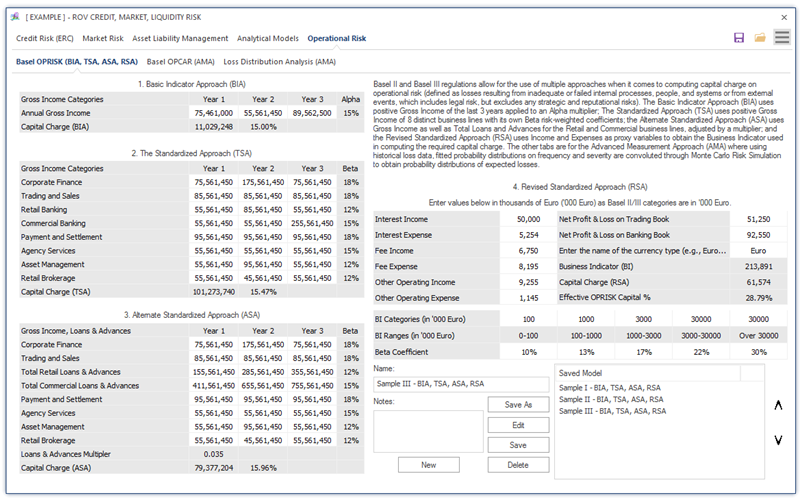
Figure 5.1: Basel III/IV BIA, TSA, ASA, RSA Methods
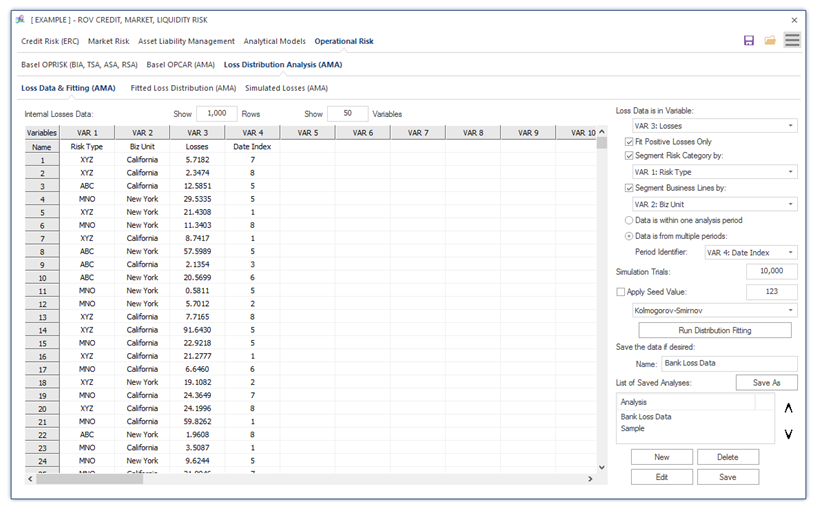
Figure 5.2: Operational Risk Data in Advanced Measurement Approach (AMA)
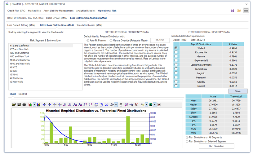
Figure 5.3: Fitted Distributions on Operational Risk Data
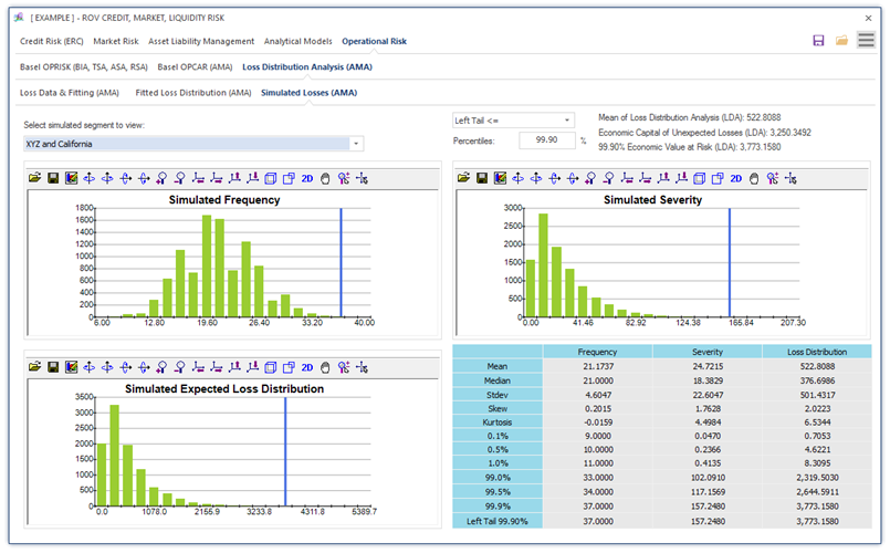
Figure 5.4: Monte Carlo Risk Simulated Operational Losses
Figure 5.5 shows the computations of Basel III/IV’s OPCAR (Operational Capital at Risk) model where the probability distribution of risk event Frequency is multiplied by the probability distribution of Severity of operational losses, the approach where Frequency × Severity is termed the Single Loss Approximation (SLA) model. The SLA is computed using convolution methods of combining multiple probability distributions. SLA using convolution methods is complex and very difficult to compute and the results are only approximations, and valid only at the extreme tails of the distribution (e.g., 99.9%). However, Monte Carlo Risk simulation provides a simpler and more powerful alternative when convoluting and multiplying two distributions of random variables to obtain the combined distribution. Clearly, the challenge is setting the relevant distributional input parameters. This is where the data-fitting and percentile-fitting tools come in handy. See Dr. Johnathan Mun’s Modeling Risk, Third Edition (Thompson–Shore) for more details.
Figure 5.6 shows the convolution simulation results where the distribution of loss frequency, severity, and expected losses are displayed. The resulting Expected Losses (EL), Unexpected Losses (UL), and Total Operational Capital at Risk (OPCAR) are also computed and shown. EL is, of course, the mean value of the simulated results, OPCAR is the tail-end 99.90th percentile, and UL is the difference between OPCAR and EL.
Figure 5.7 shows the loss severity data fitting using historical loss data. Users can paste historical loss data, select the required fitting routines (Kolmogorov–Smirnov, Akaike Criterion, Bayes Information Criterion, Anderson–Darling, Kuiper’s Statistic, etc.), and run the data-fitting routines. When in doubt, use the Kolmogorov–Smirnov routine. The best-fitting distributions, p-values, and their parameters will be listed, and the same interpretation applies as previously explained.
Figure 5.8 shows the loss severity percentile fitting instead, which is particularly helpful when there are no historical loss data and where there only exist high-level management assumptions of the probabilities certain events occur. In other words, by entering a few percentiles (%) and their corresponding values, one can obtain the entire distribution’s parameters.
These modeling tools allow smaller banks to have a first approach at more advanced operational risk management techniques. The use of internal models allows for a better calibration of regulatory capital that is knowingly overestimated for operational risk. The use of different scenarios providing various results can allow smaller banks to have a much more efficient capital allocation for operational risk that, being a Pillar I risk, tends to be quite expensive in terms of capital, and quite dangerous at the same time if capital was severely underestimated. Together with the traditional operational risk management tools, such as self-assessment and KRIs, these basic models allow for a proper IMMM risk management structure, aligned with the latest international standards.
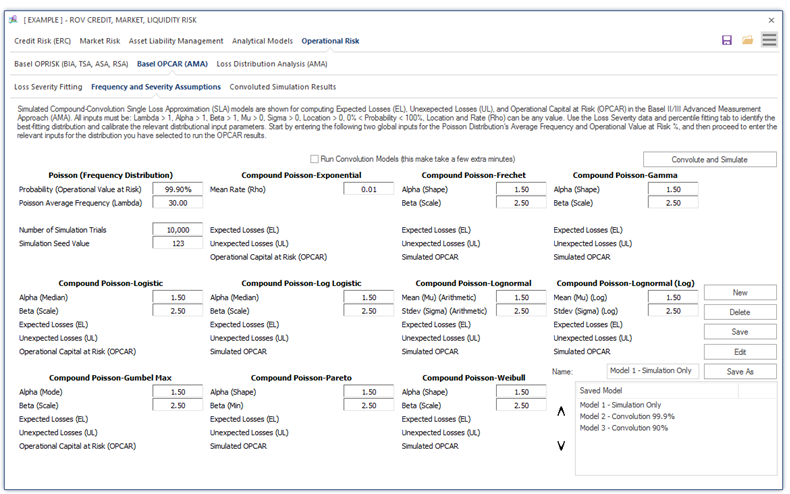
Figure 5.5: Basel OPCAR Frequency and Severity Assumptions
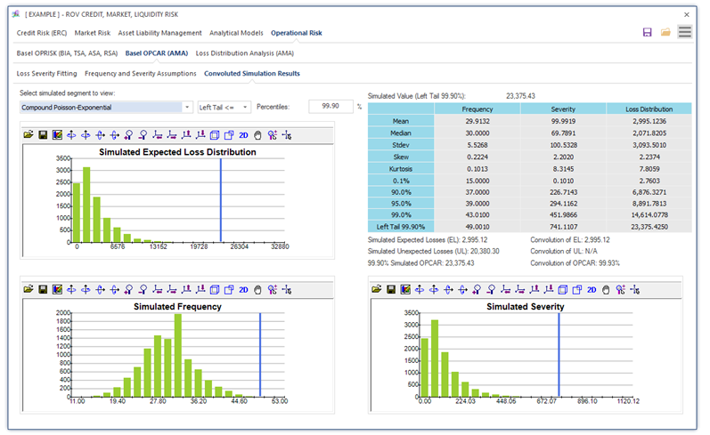
Figure 5.6: Basel OPCAR Convoluted Simulation Results
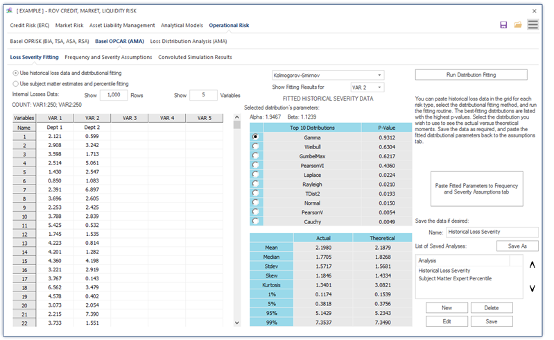
Figure 5.7: Basel OPCAR Loss Severity Data Fitting
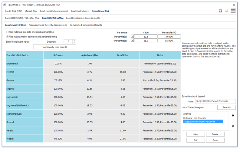
Figure 5.8: Basel OPCAR Loss Severity Percentile Fitting