File Name: Analytics – Projectile Motion
Location: Modeling Toolkit | Analytics | Projectile Motion
Brief Description: Uses simulation to compute the probabilistic distance a missile will travel given the angle of attack, initial velocity, and probability of midflight failure
Requirements: Modeling Toolkit, Risk Simulator
This example illustrates how a physics model can be built in Excel and simulated, to account for the uncertainty in inputs. This model shows the motion of a projectile (e.g., a missile) launched from the ground with a particular initial velocity, at a specific angle. The model computes the height and distance of the missile at various points in time and maps the motion in a graph. Further, we model the missile’s probability of failure (i.e., we assume that the missile can fail midflight and is a crude projectile, rather than a smart bomb, where there is no capability for any midcourse corrections and no onboard navigational and propulsion controls).
We know from physics that the location of the projectile can be mapped on an x-axis and y-axis chart, representing the distance and height of the projectile at various points in time, and those x-axis and y-axis values are determined by:
In addition, we can compute the following assuming that there is no midflight failure:
The inputs are initial velocity, angle, time step, and failure rate (Figure 5.1). Time step (delta t) is any positive value representing how granular you wish the distance and height computations to be, in terms of time. For instance, if you enter 0.10 for time steps, the time period will step 0.1 hours each period.
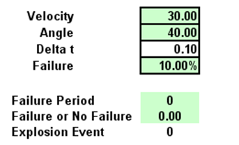
Figure 5.1: Assumptions in the missile trajectory model
Velocity, angle, and the failure rate can be uncertain and hence subject to simulation. The results are shown as a table and graphical representation. The failure rate is simulated using a Bernoulli distribution (yes-no or 0-1 distribution, with 1 representing failure, and 0 representing no failure), as seen in Figure 5.2. Figure 5.3 illustrates the sample flight path or trajectory of the missile.
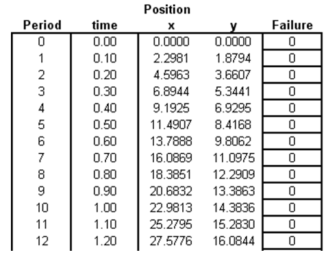
Figure 5.2: Missile coordinates midflight and probability of missile failure
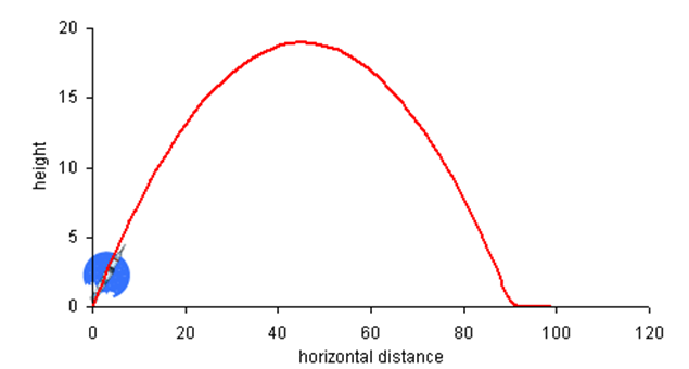
Figure 5.3 Graphical representation of the missile flight path
Procedure
This model has preset assumptions and forecasts, and is ready to be run by following these steps:
- Go to the Model worksheet and click on Risk Simulator | Change Profile and select the Projectile Motion profile.
- Run the simulation by clicking the RUN icon or Risk Simulator | Run Simulation.
- On the forecast chart, select Right-Tail, type in 110, and hit TAB on your keyboard. The results indicate that there is only a 6.80% chance that you will be hit by the missile if you lived 110 miles away, assuming all the inputs are valid (Figure 5.4).
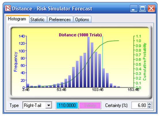
Figure 5.4: Probabilistic forecast of a projectile’s range
Alternatively, you can recreate the model assumptions and forecast by following these steps:
- Go to the Model worksheet and click on Risk Simulator | Change Profile and select the Projectile Motion profile.
- Select cell E4 and define it as an input assumption (Risk Simulator | Set Input Assumption) and choose a distribution of your choice (e.g., Normal) and click OK. Repeat for cells E5 and E7, one at a time. Then, select cell E9 and make it a Discrete Uniform distribution between 0 and 44; make cell E10 a Bernoulli distribution and click on the link icon and link it to cell E7; and make sure to check the Enable Dynamic Simulations check box and click OK (Figure 5.5).
- Select cell D60 and make it a forecast (Risk Simulator | Set Output Forecast).
- Run the simulation by clicking the RUN icon or Risk Simulator | Run Simulation.
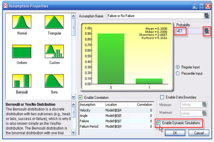
Figure 5.5: Simulating midflight failures