This Economic Results (Level 3) subtab shows the results from the chosen Project and returns the Net Present Value (NPV), Internal Rate of Return (IRR), Modified Internal Rate of Return (MIRR), Profitability Index (PI), Return on Investment (ROI), Payback Period (PP), and Discounted Payback Period (DPP), as seen in Figure 3.3. Refer to the previous chapter for details on each of the calculation methods.
An NPV Profile table and chart are also provided, where different discount rates and their respective NPV results are shown and charted. You can change the range of the discount rates to show/compute, copy the results, and copy the NPV Profile chart, as well as use any of the chart icons to manipulate the chart’s look and feel (e.g., change the chart’s line/background color, chart type, chart view, or add/remove gridlines, labels, and legend). You can also change the variable to display in the chart. For instance, you can change the chart from displaying the NPV Profile to the time-series charts of net cash flows, escalated net cash flows, taxable income, final cash flows, cumulative final cash flows, or present value of the final cash flows. You can then click on the Copy Chart button to take a screenshot of the modified chart that you can then paste into another software application such as Microsoft Excel or Microsoft PowerPoint. As a note of caution, when you click this Copy Chart button, please do give it an extra second before moving the mouse and pasting into another software because on slower computers, the native Windows imager services will need to run in the background and may take the added second or two to complete.
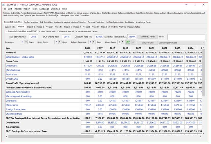
Figure 3.1 – DCF Model: Project Input Assumptions
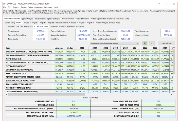
Figure 3.2 – DCF Model: Cash Flow Ratios
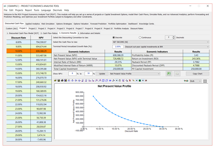
Figure 3.3 – DCF Model: Economic Results
Here are some additional tips for working in this Economic Results tab:
-
- The Economic Results are for each individual Project, whereas the Portfolio Analysis tab compares the economic results of all Projects at once.
- The Terminal Value Annualized Growth Rate is applied to the last year’s cash flow to account for a perpetual constant growth rate cash flow model, and these future cash flows are discounted back to the base year and added to the NPV to arrive at the NPV with Terminal Value result. The Gordon Growth Model is used to calculate the terminal value and then its result is discounted back to the starting year.
- You can change the Show NPV percentages and click Update to change the NPV Profile results grid and chart (assuming you selected the NPV Profile chart, as shown in Figure 3. 3).
- As usual, there are chart icons for you to modify the chart (bar chart color, chart type, chart view, background color, rotation, show/hide labels and legends, show/hide gridlines and data labels, etc.). Also available are the Copy Results and Copy Chart Again, on slower or older computers, remember to give it an additional second after you click on Copy Chart before moving the mouse and pasting into another application.
- There is a discount out-year capital investments drop-down list using the IRR Method or Discount Rate Method. The IRR result that is computed will depend on the method chosen. The traditional method is to use IRR as the reinvestment rate (default selection in the drop-down list) defined as the discount rate where the NPV = 0 (this can be verified in the NPV and Discount Rate grid on the left of the screen). This approach works in most traditional models but will return a null result if the IRR requirement is violated. IRR has a requirement that the initial Cash Flow (CF) at time 0 compared to Capital Investments (INV) at time 0 be such that INV0 > CF0, otherwise the concept of IRR and its math do not work. This method works well in most business situations (capital investments come early, and positive cash flows come later in time), but one can also have a situation where INV0 < CF0, making the Total Net Cash Flow or CF0 – INV0 > Therefore, the traditional IRR, defined as the Discount Rate where NPV = 0, will not return a valid result (this situation of the initial cash flow being greater than the investment can, in fact, occur in real-life, albeit seldom). There are two ways to solve this problem. The first is that you manually push the positive CF0 one period into the future using some discount rate or reinvestment rate or discount all future INVT amounts at the discount rate back to time zero, thereby making the Total Net Cash Flow or CF0 – INV0 < 0 as the present value of the S INVT > CF0. This is essentially the approach undertaken in the second item on the drop-down list (please be aware that in this situation, the computed IRR is really a quasi-IRR and therefore will not be the discount rate making the NPV = 0; it will, nonetheless, at least provide you a computed metric). Of course, in a highly profitable project where the present value of the S INVT < CF0, neither the traditional IRR nor the quasi-IRR works.
- IRR calculations require thatTotal Initial Cash Flow(CF0– INV < 0. This value has to be NEGATIVE.
- The IRR Method stops if (CF0 > INV0) or NET CF0 > 0. This value cannot be POSITIVE.
- The IRR Method is better in most cases except when the following occurs, then the IRR Method cannot return a value, and only the Discount Rate Method will return a result (although this is a quasi-IRR and not the traditional IRR): (CF0 > INV0) or NET CF0 > 0, and if Present Value of the S INVT > CF0.
- If Present Value of the Σ INVT < CF0, neither method works.
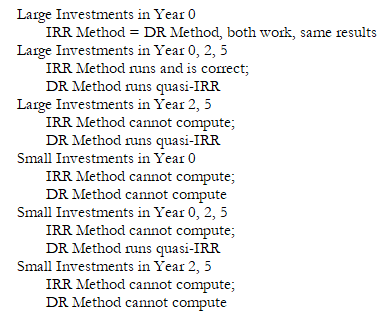
To summarize, we see the following effects on IRR calculations:
No Cash Flow at Time 0 (CF0 = 0):
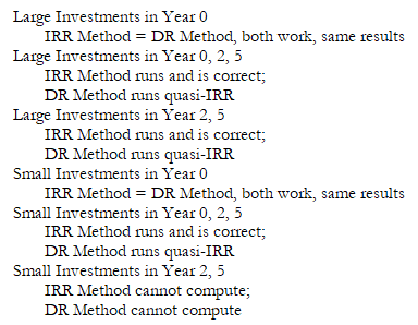
Some Cash Flow at Time 0 (CF0 > 0):