If we agree that task durations can vary, then that uncertainty should be taken into account in schedule models. A schedule model can be developed by creating a probability distribution for each task, representing the likelihood of completing the particular task at a specific duration. Monte Carlo simulation techniques can then be applied to forecast the entire range of possible project durations.
A simple triangular distribution is a reasonable probability distribution to use to describe the uncertainty for a task’s duration. It is a natural fit because if we ask someone to give a range of duration values for a specific task, he or she usually supplies two of the distribution’s elements: the minimum duration and the maximum duration. We need only ask or determine the most likely duration to complete the triangular distribution. The parameters are simple, intuitively easy to understand, and readily accepted by customers and bosses alike. Other more complex distributions could be used such as the Beta or Weibull but little, if anything, is gained because the determination of the estimated parameters for these distributions is prone to error and the method of determination is not easily explainable to the customer or boss.
To get the best estimates, we should use multiple sources to get the estimates of the minimum, most likely, and maximum values for the task durations. We can talk to the contractor, the project manager, and the people doing the hands-on work and then compile a list of duration estimates. Historical data can also be used, but with caution, because many efforts may be similar to past projects but usually contain several unique elements or combinations. We can use Figure 1.2 as a guide. Minimum values should reflect optimal utilization of resources. Maximum values should take into account substantial problems, but it is not necessary to account for the absolute worst case where everything goes wrong, and the problems compound each other. Note that the most likely value will be the value experienced most often, but it is typically less than the median or mean in most cases. For our example problem, shown in Figure 1.1, the minimum, most likely, and maximum values given in Figure 1.3 will be used. We can use Risk Simulator’s input assumptions to create triangular distributions based on these minimum, most likely, and maximum parameters. The column of dynamic duration values shown in Figure 1.3 was created by taking one random sample from each of the associated triangular distributions.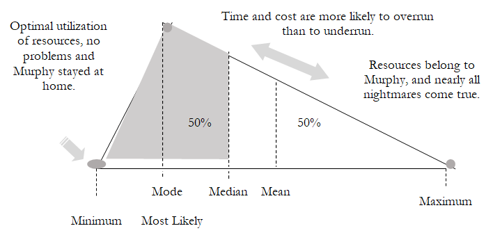
Figure 1.2: Triangular Distribution
After the triangular distributions are created, the next step is to use the schedule network to determine the paths. For the example problem shown in Figure 1.1, there are four paths through the network from beginning to end. These paths are shown in Figure 1.4 with their associated durations. (Note: When setting up the spreadsheet for the various paths, it is absolutely essential to use the input assumptions for the task durations and then reference these task duration cells when calculating the duration for each path. This method ensures that the duration of individual tasks is the same regardless of which path is used.) The overall schedule total duration is the maximum of the four paths. In Risk Simulator, we would designate that cell as an Output Forecast. In probabilistic schedule analysis, we are not concerned with the critical path/near-critical path situations because the analysis automatically accounts for all path durations through the calculations.
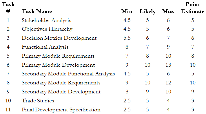
Figure 1.3: Range of Task Durations
We can now use Risk Simulator and run a Monte Carlo simulation to produce a forecast for schedule duration. Figure 1.5 shows the results for the example problem. Let us return to the numbers given by the traditional method. The original estimate stated the project would be complete in 37 days. If we use the left-tail function on the forecast chart, we can determine the likelihood of completing the task in 37 days based on the Monte Carlo simulation. In this case, there is a mere 8.27% chance of completion within the 37 days. This result illustrates the second shortcoming in the traditional method: Not only is the point estimate incorrect, but it puts us in a high-risk overrun situation before the work has even started! As shown in Figure 1.5, the median value is 38.5 days. Some industry standards recommend using the 80% certainty value for most cases, which equates to 39.5 days in the example problem.
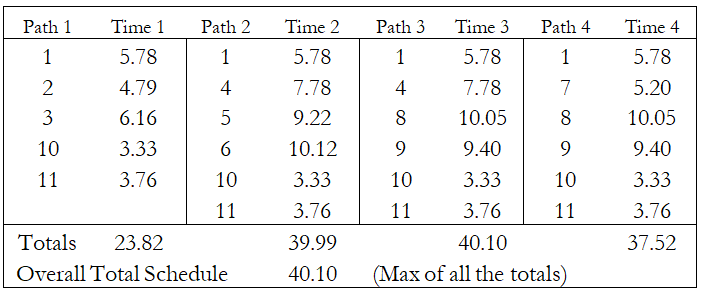
Figure 1.4: Paths and Durations for Example Problem
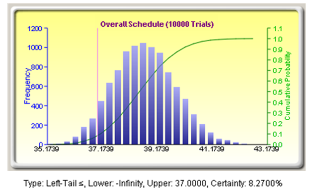
Figure 1.5: Simulation Results
Now let us revisit the boss’s request to reduce the whole schedule by one day. Where do we put the effort to reduce the overall duration? If we are using probabilistic schedule management, we do not use the critical path; so, where do we start? Using Risk Simulator’s Tornado Analysis and Sensitivity Analysis tools, we can identify the most effective targets for reduction efforts. The tornado chart (Figure 1.6) identifies the most influential variables (tasks) to the overall schedule. This chart provides the best targets to reduce the mean/median values.

Figure 1.6: Tornado Analysis
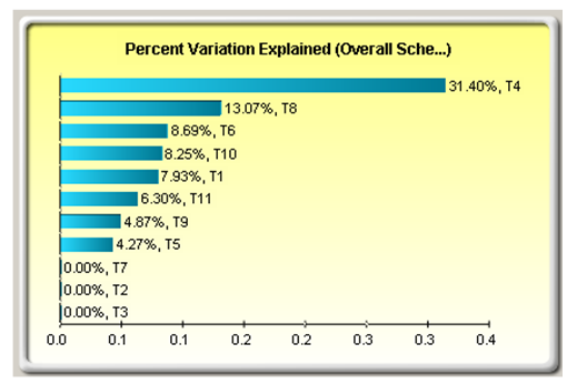
Figure 1.7: Sensitivity Analysis
We cannot address the mean/median without addressing the variation, however. The Sensitivity Analysis tool shows what variables (tasks) contribute the most to the variation in the overall schedule output (see Figure 1.7). In this case, we can see that the variation in Task 4 is the major contributor to the variation in the overall schedule. Another interesting observation is that the variation in Task 6, a task not on the critical path, is also contributing nearly 9% of the overall variation.
In this example, reducing the schedule duration for Task 4, Task 8, and Task 9 would pay the most dividends as far as reducing the overall schedule length. Determining the underlying reasons for the substantial variation in Tasks 4, 6, and 8 would likely give better insight into these processes. For example, the variation in Task 4 may be caused by the lack of available personnel. Management actions could be taken to dedicate personnel to the effort and reduce the variation substantially, which would reduce the overall variation and enhance the predictability of the schedule. Digging into the reasons for variation will lead to targets where management actions will be most effective, much more so than by simply telling the troops to reduce their task completion time.
Using the network schedule model, we can also experiment to see how different reduction strategies may pay off. For example, taking one day out of Tasks 4, 8, and 9 under the traditional method would lead us to believe that a three-day reduction has taken place, but if we reduce the Most Likely value for Tasks 4, 8, and 9 by one day and run the Monte Carlo risk simulation, we find that the median value is still 37.91, or only a 0.7-day reduction. This small reduction proves that the variation must be addressed. If we reduce the variation by 50%, keeping the original minimum and the most likely values, but reducing the maximum value for each distribution, then we reduce the median from 38.5 to 37.91—about the same as reducing the most likely values. Taking both actions (reducing the most likely and maximum values) reduces the median to 36.83, giving us a 55% chance of completing within 37 days. This analysis proves that reducing the most likely value and the overall variation is the most effective action.
To get to 36 days, we need to continue to work down the list of tasks shown in the sensitivity and tornado charts addressing each task. If we give Task 1 the same treatment, reducing its most likely and maximum values, then completion within 36 days can be accomplished with a 51% certainty and a 79.25% certainty of completing within 37 days. The maximum value for the overall schedule is reduced from more than 42 days to less than 40 days. Substantial management efforts would be needed, however, to reach 36 days at the 80% certainty level.
When managing the production schedule, use the best-case numbers. If we use the most likely values or, worse yet, the maximum values, production personnel will not strive to hit the best-case numbers thus implementing a self-fulfilling prophecy of delayed completion. When budgeting, we should create the budget for the median outcome but recognize that there is uncertainty in the real world as well as risk. When relating the schedule to the customer, provide the values that equate to the 75% to 80% certainty level. In most cases, customers prefer predictability (on-time completion) over potentially speedy completion that includes significant risk. Lastly, acknowledge that the “worst case” can conceivably occur and create contingency plans to protect your organization in case it does occur. If the “worst case”/maximum value is unacceptable, then make the appropriate changes in the process to reduce the maximum value of the outcome to an acceptable level.
Conclusion
With traditional schedule management, there is only one answer for the scheduled completion date. Each task gets one duration estimate and that estimate is accurate only if everything goes according to plan, which is not a likely occurrence. With probabilistic schedule management, thousands of trials are run exploring the range of possible outcomes for schedule duration. Each task in the network receives a time estimate distribution, accurately reflecting each task’s uncertainty. Correlations can be entered to more accurately model real-world behavior. Critical paths and near-critical paths are automatically taken into account, and the output forecast distribution will accurately reflect the entire range of possible outcomes. Using tornado and sensitivity analyses, we can maximize the effectiveness of our management actions to control schedule variations and, if necessary, reduce the overall schedule at high certainty levels.