The regression and forecasting diagnostic tool is the advanced analytical tool in Risk Simulator used to determine the econometric properties of your data. The diagnostics include checking the data for heteroskedasticity, nonlinearity, outliers, specification errors, micronumerosity, stationarity and stochastic properties, normality and sphericity of the errors, and multicollinearity. Each test is described in more detail in their respective reports in the model.
Procedure
- Open the example model(Risk Simulator | Example Models | Regression Diagnostics), and go to the Time-Series Data worksheet, and select the data including the variable names (cells C5:H55).
- Click on Risk Simulator | Analytical Tools | Diagnostic Tool.
- Check the data and select the Dependent Variable Y from the drop-down menu. Click OK when finished (Figure 12.48).
A common violation in forecasting and regression analysis is heteroskedasticity; that is, the variance of the errors increases over time (see Figure 12.49 for test results using the diagnostic tool). Visually, the width of the vertical data fluctuations increases or fans out over time, and, typically, the coefficient of determination (R-squared coefficient) drops significantly when heteroskedasticity exists. If the variance of the dependent variable is not constant, then the error’s variance will not be constant. Unless the heteroskedasticity of the dependent variable is pronounced, its effect will not be severe: The least-squares estimates will still be unbiased, and the estimates of the slope and intercept will either be normally distributed if the errors are normally distributed or at least normally distributed asymptotically (as the number of data points becomes large) if the errors are not normally distributed. The estimate for the variance of the slope and overall variance will be inaccurate, but the inaccuracy is not likely to be substantial if the independent-variable values are symmetric about their mean.
If the number of data points is small (micronumerosity), it may be difficult to detect assumption violations. With small sample sizes, assumption violations such as non-normality or heteroskedasticity of variances are difficult to detect even when they are present. With a small number of data points, linear regression offers less protection against the violation of assumptions. With few data points, it may be hard to determine how well the fitted line matches the data, or whether a nonlinear function would be more appropriate. Even if none of the test assumptions are violated, a linear regression on a small number of data points may not have sufficient power to detect a significant difference between the slope and zero, even if the slope is nonzero. The power depends on the residual error, the observed variation in the independent variable, the selected significance alpha level of the test, and the number of data points. Power decreases as the residual variance increases, decreases as the significance level is decreased (i.e., as the test is made more stringent), increases as the variation in observed independent variable increases, and increases as the number of data points increases.
Values may not be identically distributed because of the presence of outliers. Outliers are anomalous values in the data. Outliers may have a strong influence over the fitted slope and intercept, giving a poor fit to the bulk of the data points. Outliers tend to increase the estimate of residual variance, lowering the chance of rejecting the null hypothesis; that is, creating higher prediction errors. They may be due to recording errors, which may be correctable, or they may be due to the dependent-variable values not all being sampled from the same population. Apparent outliers may also be due to the dependent-variable values being from the same, but non-normal, population. However, a point may be an unusual value in either an independent or dependent variable without necessarily being an outlier in the scatter plot. In regression analysis, the fitted line can be highly sensitive to outliers. In other words, least squares regression is not resistant to outliers, thus, neither is the fitted-slope estimate. A point vertically removed from the other points can cause the fitted line to pass close to it, instead of following the general linear trend of the rest of the data, especially if the point is relatively far horizontally from the center of the data.
![]()
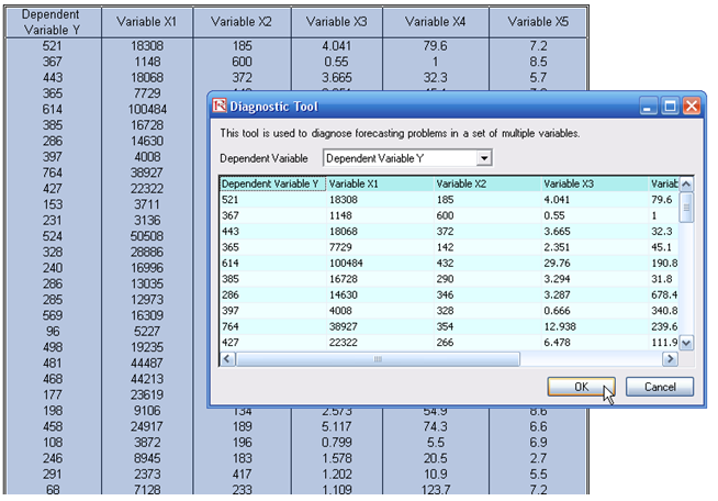
Figure 12.48: Running the Data Diagnostic Tool
However, great care should be taken when deciding if the outliers should be removed. Although in most cases when outliers are removed, the regression results look better, a priori justification must first exist. For instance, if one is regressing the performance of a particular firm’s stock returns, outliers caused by downturns in the stock market should be included; these are not truly outliers as they are inevitabilities in the business cycle. Forgoing these outliers and using the regression equation to forecast one’s retirement fund based on the firm’s stocks will yield incorrect results at best. In contrast, suppose the outliers are caused by a single nonrecurring business condition (e.g., merger and acquisition) and such business structural changes are not forecast to recur; then these outliers should be removed and the data cleansed prior to running a regression analysis. The analysis here only identifies outliers and it is up to the user to determine if they should remain or be excluded.
Sometimes, a nonlinear relationship between the dependent and independent variables is more appropriate than a linear relationship. In such cases, running a linear regression will not be optimal. If the linear model is not the correct form, then the slope and intercept estimates and the fitted values from the linear regression will be biased, and the fitted slope and intercept estimates will not be meaningful. Over a restricted range of independent or dependent variables, nonlinear models may be well approximated by linear models (this is, in fact, the basis of linear interpolation), but for accurate prediction, a model appropriate to the data should be selected. A nonlinear transformation should first be applied to the data before running a regression. One simple approach is to take the natural logarithm of the independent variable (other approaches include taking the square root or raising the independent variable to the second or third power) and run a regression or forecast using the nonlinearly transformed data.
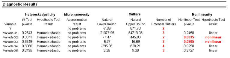
Figure 12.49: Results from Tests of Outliers, Heteroskedasticity, Micronumerosity, and Nonlinearity
Another typical issue when forecasting time-series data is whether the independent-variable values are truly independent of each other or are actually dependent. Dependent variable values collected over a time series may be autocorrelated. For serially correlated dependent-variable values, the estimates of the slope and intercept will be unbiased, but the estimates of their forecast and variances will not be reliable and, hence, the validity of certain statistical goodness-of-fit tests will be flawed. For instance, interest rates, inflation rates, sales, revenues, and many other time-series data are typically autocorrelated, where the value in the current period is related to the value in a previous period, and so forth (clearly, the inflation rate in March is related to February’s level, which, in turn, is related to January’s level, etc.). Ignoring such blatant relationships will yield biased and less accurate forecasts. In such events, an autocorrelated regression model or an ARIMA model may be better suited (Risk Simulator | Forecasting | ARIMA). Finally, the autocorrelation functions of a series that is nonstationary tend to decay slowly (see nonstationary report in the model).
If autocorrelation AC(1) is nonzero, it means that the series is first-order serially correlated. If AC(k) dies off more or less geometrically with increasing lag, it implies that the series follows a low-order autoregressive process. If AC(k) drops to zero after a small number of lags, it implies that the series follows a low-order moving average process. Partial correlation PAC(k) measures the correlation of values that are k periods apart after removing the correlation from the intervening lags. If the pattern of autocorrelation can be captured by an autoregression of order less than k, then the partial autocorrelation at lag k will be close to zero. Ljung–Box Q-statistics and their p-values at lag k have the null hypothesis that there is no autocorrelation up to order k. The dotted lines in the plots of the autocorrelations are the approximate two standard error bounds. If the autocorrelation is within these bounds, it is not significantly different from zero at the 5% significance level.
Autocorrelation measures the relationship to the past of the dependent Y variable to itself. Distributive lags, in contrast, are time-lag relationships between the dependent Y variable and different independent X variables. For instance, the movement and direction of mortgage rates tend to follow the Federal Funds Rate but at a time lag (typically 1 to 3 months). Sometimes, time lags follow cycles and seasonality (e.g., ice-cream sales tend to peak during the summer months and are therefore related to last summer’s sales, 12 months in the past). The distributive lag analysis (Figure 12.50) shows how the dependent variable is related to each of the independent variables at various time lags, when all lags are considered simultaneously, to determine which time lags are statistically significant and should be considered.
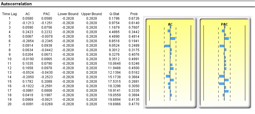
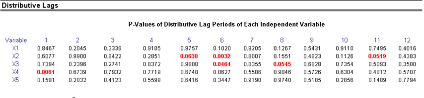
Figure 12.50: Autocorrelation and Distributive Lag Results
Another requirement in running a regression model is the assumption of normality and sphericity of the error term. If the assumption of normality is violated or outliers are present, then the linear regression goodness-of-fit test may not be the most powerful or informative test available. Choosing the most appropriate test could mean the difference between detecting a linear fit or not. If the errors are not independent and not normally distributed, it may indicate that the data might be autocorrelated or suffer from nonlinearities or other more destructive errors. Independence of the errors can also be detected in the heteroskedasticity tests (Figure 12.51).
The normality test on the errors performed is a nonparametric test, which makes no assumptions about the specific shape of the population from where the sample is drawn, allowing for smaller sample datasets to be analyzed. This test evaluates the null hypothesis of whether the sample errors were drawn from a normally distributed population versus an alternate hypothesis that the data sample is not normally distributed. If the calculated D-statistic is greater than or equal to the D-critical values at various significance values, then reject the null hypothesis and accept the alternate hypothesis (the errors are not normally distributed). Otherwise, if the D-statistic is less than the D-critical value, do not reject the null hypothesis (the errors are normally distributed). This test relies on two cumulative frequencies: one derived from the sample dataset and the second from a theoretical distribution based on the mean and standard deviation of the sample data.
Sometimes, certain types of time-series data cannot be modeled using any other methods except for a stochastic process, because the underlying events are stochastic in nature. For instance, you cannot adequately model and forecast stock prices, interest rates, price of oil, and other commodity prices using a simple regression model because these variables are highly uncertain and volatile, and do not follow a predefined static rule of behavior; in other words, the process is not stationary. Stationarity is checked here using the Runs Test, while another visual clue is found in the Autocorrelation report (the ACF tends to decay slowly). A stochastic process is a sequence of events or paths generated by probabilistic laws. That is, random events can occur over time but are governed by specific statistical and probabilistic rules. The main stochastic processes include a random walk or Brownian motion, mean reversion, and jump-diffusion. These processes can be used to forecast a multitude of variables that seemingly follow random trends but are restricted by probabilistic laws. The process-generating equation is known in advance, but the actual results generated are unknown (Figure 12.52).
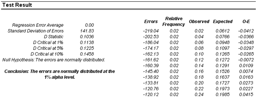
Figure 12.51: Test for Normality of Errors
The random walk Brownian motion process can be used to forecast stock prices, prices of commodities, and other stochastic time-series data given a drift or growth rate and volatility around the drift path. The mean-reversion process can be used to reduce the fluctuations of the random walk process by allowing the path to target a long-term value, making it useful for forecasting time-series variables that have a long-term rate such as interest rates and inflation rates (these are long-term target rates by regulatory authorities or the market). The jump-diffusion process is useful for forecasting time-series data when the variable can occasionally exhibit random jumps, such as oil prices or the price of electricity (discrete exogenous event shocks can make prices jump up or down). These processes can also be mixed and matched as required.
A note of caution is required here. The stochastic parameters calibration shows all the parameters for all processes and does not distinguish which process is better and which is worse or which process is more appropriate to use. It is up to the user to make this determination. For instance, if we see a 283% reversion rate, chances are a mean-reversion process is inappropriate, or a very high jump rate of, say, 100% most probably means that a jump-diffusion process is probably not appropriate, and so forth. Further, the analysis cannot determine what the variable is and what the data source is. For instance, is the raw data from historical stock prices, or is it the historical prices of electricity or inflation rates or the molecular motion of subatomic particles, and so forth. Only the user would know such information, and, hence, using a priori knowledge and theory, be able to pick the correct process to use (e.g., stock prices tend to follow a Brownian motion random walk whereas inflation rates follow a mean-reversion process, or a jump-diffusion process is more appropriate should you be forecasting the price of electricity).
Multicollinearity exists when there is a linear relationship between the independent variables. When this occurs, the regression equation cannot be estimated at all. In near collinearity situations, the estimated regression equation will be biased and provide inaccurate results. This situation is especially true when a step-wise regression approach is used, where the statistically significant independent variables will be thrown out of the regression mix earlier than expected, resulting in a regression equation that is neither efficient nor accurate. One quick test of the presence of multicollinearity in a multiple regression equation is that the R-squared value is relatively high while the t-statistics are relatively low.
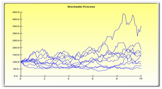
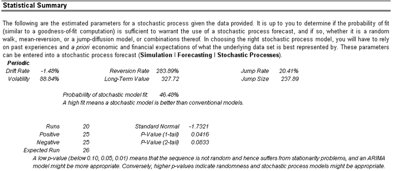
Figure 12.52: Stochastic Process Parameter Estimation
Another quick test is to create a correlation matrix between the independent variables. A high cross-correlation indicates a potential for autocorrelation. The rule of thumb is that a correlation with an absolute value greater than 0.75 is indicative of severe multicollinearity. Another test for multicollinearity is the use of the Variance Inflation Factor (VIF), obtained by regressing each independent variable to all the other independent variables, obtaining the R-squared value, and calculating the VIF. A VIF exceeding 2.0 can be considered as severe multicollinearity. A VIF exceeding 10.0 indicates destructive multicollinearity (Figure 12.53).
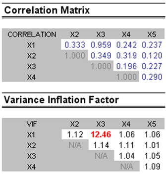
Figure 12.53: Multicollinearity Errors
The correlation matrix lists the Pearson’s product-moment correlations (commonly referred to as the Pearson’s R) between variable pairs. The correlation coefficient ranges between –1.0 and + 1.0, inclusive. The sign indicates the direction of association between the variables, while the coefficient indicates the magnitude or strength of association. The Pearson’s R only measures a linear relationship and is less effective in measuring nonlinear relationships.
To test whether the correlations are significant, a two-tailed hypothesis test is performed and the resulting p-values are computed. P-values less than 0.10, 0.05, and 0.01 are highlighted in blue to indicate statistical significance. In other words, a p-value for a correlation pair that is less than a given significance value is statistically significantly different from zero, indicating that there is a significant linear relationship between the two variables.
The Pearson’s product-moment correlation coefficient (R) between two variables (x and y) is related to the covariance (cov) measure where
The benefit of dividing the covariance by the product of the two variables’ standard deviations (s) is that the resulting correlation coefficient is bounded between –1.0 and +1.0, inclusive. This parameter makes the correlation a good relative measure to compare among different variables (particularly with different units and magnitude). The Spearman rank-based nonparametric correlation is also included in the analysis. The Spearman’s R is related to the Pearson’s R in that the data is first ranked and then correlated. The rank correlations provide a better estimate of the relationship between two variables when one or both of them is nonlinear.
It must be stressed that a significant correlation does not imply causation. Associations between variables in no way imply that the change of one variable causes another variable to change. Two variables that are moving independently of each other but in a related path may be correlated but their relationship might be spurious (e.g., a correlation between sunspots and the stock market might be strong, but one can surmise that there is no causality and that this relationship is purely spurious).