File Names: Real Options – Simple Two-Phased Sequential Compound Option; Real Options – Multiple-Phased Sequential Compound Option; Real Options – Multiple-Phased Complex Sequential Compound Option
Location: Modeling Toolkit | Real Options Models
Brief Description: Computes sequential compound options with multiple-phased and complex interrelationships between phases and customizable and changing input parameters
Requirements: Modeling Toolkit, Real Options SLS
Sequential Compound Options are applicable for research and development investments or any other investments that have multiple stages. The Real Options SLS software is required for solving Sequential Compound Options. The easiest way to understand this option is to start with a two-phased example as seen in Figure 191.1. In a two-phased example, management has the ability to decide if Phase II (PII) should be implemented after obtaining the results from Phase I (PI). For example, a pilot project or market research in PI indicates that the market is not yet ready for the product, hence PII is not implemented. All that is lost is the PI sunk cost, not the entire investment cost of both PI and PII. The next section illustrates how the option is analyzed.
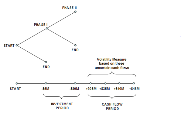 Figure 191.1: Graphical representation of a two-phased sequential compound option
Real Options – Simple Two-Phased Sequential Compound Option
Figure 191.1 is valuable in explaining and communicating to senior management the aspects of an American Sequential Compound Option and its inner workings. In the illustration, the Phase I investment of –$5M (in present value dollars) in Year 1 is followed by Phase II investment of –$80M (in present value dollars) in Year 2. It is hoped that positive net free cash flows (CF) will follow in Years 3 to 6, yielding a sum of PV Asset of $100M (CF discounted at, say, a 9.7% discount or hurdle rate), and the Volatility of these CFs is 30%. At a 5% risk-free rate, the strategic value is calculated at $27.67 as seen in Figure 191.2 using a 100-step lattice, which means that the strategic option value of being able to defer investments and to wait and see until more information becomes available and uncertainties become resolved is worth $12.67M because the NPV is worth $15M ($100M – $5M – $80M). In other words, the Expected Value of Perfect Information is worth $12.67M, which indicates that if market research can be used to obtain credible information to decide if this project is a good one, the maximum the firm should be willing to spend in Phase I is on average no more than $17.67M (i.e., $12.67M + $5M) if PI is part of the market research initiative, or simply $12.67M otherwise. If the cost to obtain the credible information exceeds this value, then it is optimal to take the risk and execute the entire project immediately at $85M. The example file used is Simple Two-Phased Sequential Compound Option.
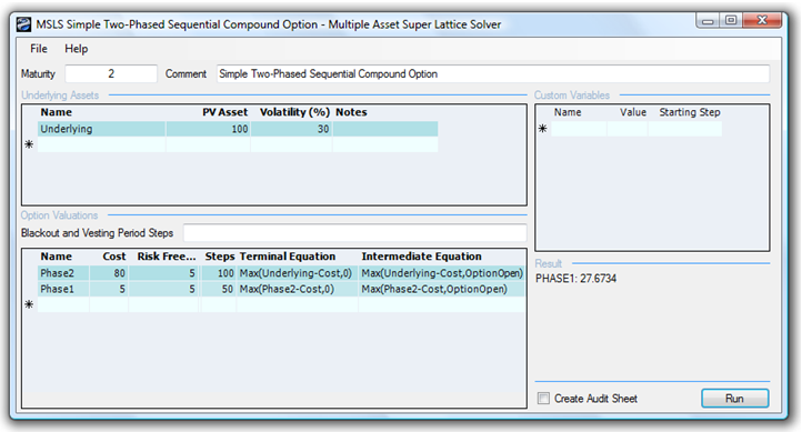
Figure 191.2: Solving a two-phased sequential compound option using SLS
In contrast, if the volatility decreases (uncertainty and risk are lower), the strategic option value decreases. In addition, when the cost of waiting (as described by the Dividend Rate as a percentage of the Asset Value) increases, it is better not to defer and wait that long. Therefore, the higher the dividend rate, the lower the strategic option value. For instance, at an 8% dividend rate and 15% volatility, the resulting value reverts to the NPV of $15M, which means that the option value is zero, and that it is better to execute immediately as the cost of waiting far outstrips the value of being able to wait given the level of volatility (uncertainty and risk). Finally, if risks and uncertainty increase significantly even with a high cost of waiting (e.g., 7% dividend rate at 30% volatility), it is still valuable to wait.
This model provides the decision maker with a view into the optimal balancing between waiting for more information (Expected Value of Perfect Information) and the cost of waiting. You can analyze this balance by creating strategic options to defer investments through development stages where at every stage the project is reevaluated as to whether it is beneficial to proceed to the next phase. Based on the input assumptions used in this model, the Sequential Compound Option results show the strategic value of the project, and the NPV is simply the PV Asset less the Implementation Costs of both phases. In other words, the strategic option value is the difference between the calculated strategic value minus the NPV. It is recommended that you vary the volatility and dividend inputs to determine their interactions—specifically, where the break-even points are for different combinations of volatilities and dividends. Using this information, you can make better go or no-go decisions based on the resulting option value (for instance, break-even volatility points can be traced back into the discounted cash flow model to estimate the probability of crossing over and this ability to wait becomes valuable).
Note that the investment costs of $80M and $5M are in present values for several reasons. The first is that only the PV Asset undergoes an underlying asset lattice evolution to future values; costs do not undergo such an evolution, and are hence in present values. Also, for example, in a five-year option, an implementation that can occur at any time within these five years will have very different actual implementation costs. To make these costs comparable, we use their present values. Thus, an $80M cost can occur at any time within some specified time period; the present value of the cost is still $80M regardless of when it hits. Finally, the risk-free rate discounts the expected value of keeping the option open, not the cost. So, there is no double-discounting and using the present value for these costs is correct.
Real Options – Multiple-Phased Sequential Compound Option
The Sequential Compound Option can similarly be extended to multiple phases with the use of the SLS software. A graphical representation of a multi-phased or stage-gate investment is seen in Figure 191.3. The example illustrates a ten-phase project, where, at every phase, management has the option and flexibility either to continue to the next phase if everything goes well, or to terminate the project otherwise. Based on the input assumptions, the results in the SLS indicate the calculated strategic value of the project, while the NPV of the project is simply the PV Asset less all Implementation Costs (in present values) if implementing all phases immediately. Therefore, with the strategic option value of being able to defer and wait before implementing future phases (due to the volatility, there is a possibility that the asset value will be significantly higher) the strategic value of the project is higher. Hence, the ability to wait before making the investment decisions in the future is the option value or the strategic value of the project less the NPV.
Figure 191.4 shows the results using the SLS software. Notice that due to the backward induction process used, the analytical convention is to start with the last phase and go all the way back to the first phase (example file used: Multiple Phased Sequential Compound Option). In NPV terms the project is worth –$500. However, the total strategic value of the stage-gate investment option is worth $41.78. This means that although the investment looks bad on an NPV basis, in reality, by hedging the risks and uncertainties through sequential investments, the option holder can pull out at any time and not have to keep investing unless things look promising. If after the first phase things look bad, the option holder can pull out and stop investing; the maximum loss will be $100 (Figure 191.4), not the entire $1,500 investment. If, however, things look promising, the option holder can continue to invest in stages. The expected value of the investments in present values after accounting for the probabilities that things will look bad (and hence stop investing) versus things looking great (and hence continuing to invest) is worth an average of $41.78M.
Notice that the option valuation result will always be greater than or equal to zero (e.g., try reducing the volatility to 5% and increasing the dividend yield to 8% for all phases). When the option value is very low or zero, this means that it is not optimal to defer investments. The stage-gate investment process is not optimal here. The cost of waiting is too high (high dividend) or the uncertainties in the cash flows are low (low volatility); hence, invest if the NPV is positive. In such a case, although you obtain a zero value for the option, the analytical interpretation is significant! A zero or very low value is indicative of an optimal decision not to wait.
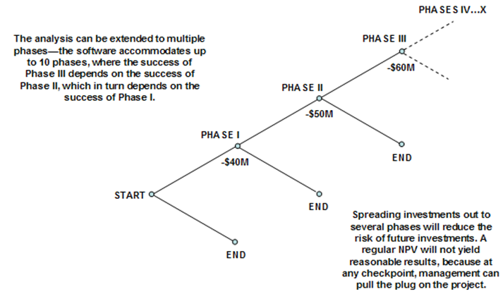
Figure 191.3: Graphical representation of a multi-phased sequential compound option
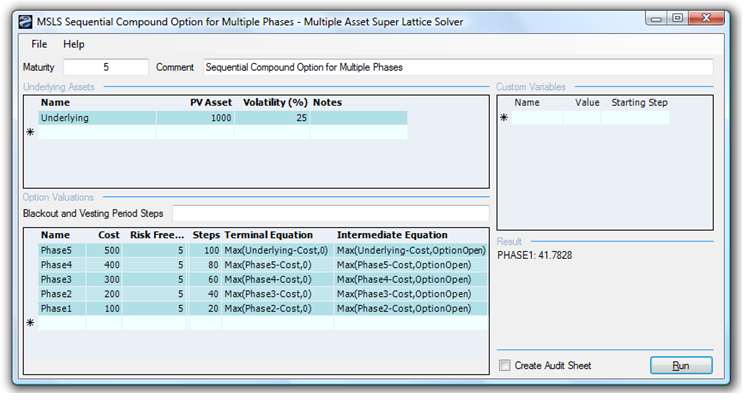
Figure 191.4: Solving a multi-phased sequential compound option using SLS
Real Options – Multiple-Phased Complex Sequential Compound Option
The Sequential Compound Option can be further complicated by adding customized options at each phase as illustrated in Figure 191.5. In the figure, at every phase, there may be different combinations of mutually exclusive options including the flexibility to stop investing, abandon and salvage the project in return for some value, expand the scope of the project into another project (e.g., spin-off projects and expand into different geographical locations), contract the scope of the project resulting in some savings, or continue on to the next phase. The seemingly complicated option can be very solved easily using SLS as seen in Figure 191.6 (example file used: Real Options – Multiple Phased Complex Sequential Compound Option).
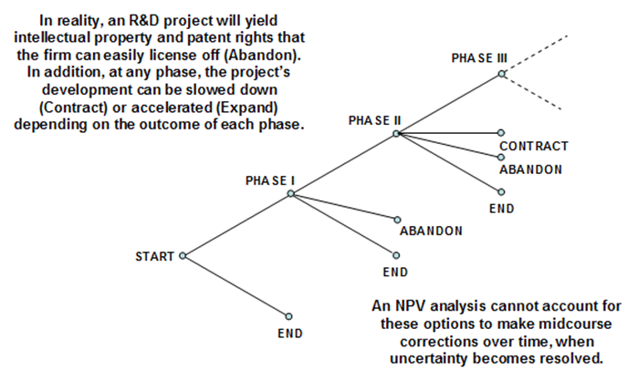
Figure 191.5: Graphical representation of a complex multi-phased sequential compound option
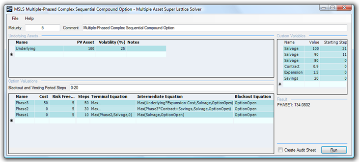
Figure 191.6: Solving a complex multi-phased sequential compound option using SLS
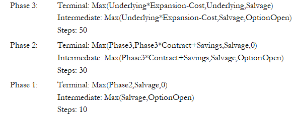
To illustrate, Figure 191.6’s SLS path-dependent sequential option uses the following inputs:
Exercise: Sequential Compound Option
A sequential compound option exists when a project has multiple phases and the latter phases depend on the success of previous ones. Suppose a project has two phases, of which the first has a one-year expiration that costs $500 million. The second phase’s expiration is three years and costs $700 million. Suppose that the implied volatility of the logarithmic returns on the projected future cash flows is calculated to be 20%. The risk-free rate on a riskless asset for the next three years is found to be yielding 7.7%. The static valuation of future profitability using a discounted cash flow model—in other words, the present value of the future cash flows discounted at an appropriate market risk-adjusted discount rate—is found to be $1,000 million. Do the following exercises, answering the questions posed:
- Solve the sequential compound option problem manually using a 10-step lattice and confirm the results by generating an audit sheet using the software.
- Change the sequence of the costs. That is, set the first phase’s cost to $700 and the second phase’s cost to $500 (both in present values). Compare your results. Explain what happens.
- Now suppose the total cost of $1,200 (in present values) is spread out equally over six phases in six years. How would the analysis results differ?
- Suppose that the project is divided into three phases with the following options in each phase as described. Solve the option using Multiple Asset SLS.
- Phase 3 occurs in three years, the implementation cost is $300, but the project can be abandoned and salvaged to receive $300 at any time within the first year, $350 within the second year, and $400 within the third year.
- Phase 2 occurs in two years, and the project can be spun off to a partner. In doing this, the partner keeps 15% of the NPV and saves the firm $200.
- Phase 1 occurs in one year, and the only thing that can be done is to invest the $300 implementation cost and continue to the next phase.