File Name: Analytics – Mathematical Integration Approximation Model
Location: Modeling Toolkit | Analytics | Mathematical Integration Approximation Model
Brief Description: Applies simulation to estimate the area under a curve without the use of any calculus-based mathematical integration
Requirements: Modeling Toolkit, Risk Simulator
Theoretical Background
There are several ways to compute the area under a curve. The best approach is the mathematical integration of a function or equation. For instance, if you have the equation:

then the area under the curve between 1 and 10 is found through the integral:
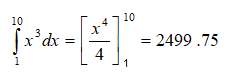
Similarly, any function f(x) can be solved and found this way. However, for complex functions, applying mathematical integration might be somewhat cumbersome. This is where simulation comes in. To illustrate, how would you solve a seemingly simple problem like the following?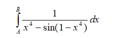
Well, dust off those old, advanced calculus books and get the solution:
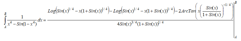
The point is sometimes simple-looking functions get really complicated. Using Monte Carlo simulation, we can approximate the value under the curve. Note that this approach yields only approximations, not exact values. Let’s see how this approach works…
The area under a curve can be seen as the shaded area (A.T.R.U.B) in Figure 4.1, between the x-axis values of A and B, and the y = f(x) curve.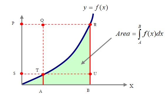
Figure 4.1: Graphical representation of a mathematical integration
Looking closely at the graph, one can actually imagine two boxes. Specifically, if the area of interest is the shaded region or A.T.R.U.B, then we can draw two imaginary boxes, A.T.U.B and T.Q.R.U. Computing the area of the first box is simple, where we have a simple rectangle. Computing the second box is trickier, as part of the area in the box is below the curve and part of it is above the curve. In order to obtain the area under the curve that is within the T.Q.R.U box, we run a simulation with a uniform distribution between the values A and B, and compute the corresponding values on the y-axis using the f(x) function, while at the same time, simulate a uniform distribution between f(A) and f(B) on the y-axis. Then we find the average number of times the simulated values on the y-axis are at or below the curve or f(x) value. Using this average value, we multiply it by the area in the box to approximate the value under the curve in the box. Summing this value with the smaller box of A.T.U.B provides the entire area under the curve.
Model Background
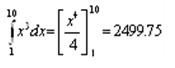
The analysis in the Model worksheet illustrates an approximation of a simple equation; namely, we have the following equation to value:

Solving this integration, we obtain the value under the curve of:
Now, we attempt to solve this using simulation through the model shown in Figure 4.2.
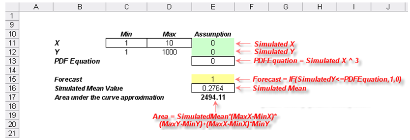
Figure 4.2: Simulation model for mathematical integration
Procedure
- We first enter the minimum and maximum values on the x-axis. In this case, they are 1 and 10 (cells C11 and D11 in Figure 4.2). This represents the range on the x-axis we are interested in.
- Next, compute the corresponding y-axis values(cells C12 and D12). For instance, in this example we have y = f(x) = x3, which means that for x = 1, we have y = 13 = 1 and for x = 10, we have y = 103 = 1000.
- Set two uniform distribution assumptions between the minimum and maximum values, one for x and one for y (cells E11 and E12).
- Compute the PDF equation, in this example, it is y = f(x) = x3 in cell E13, linking the x value in the equation to the simulated x value.
- Create a dummy 0,1 variable and set it as IF(SimulatedY <= PDFEquation, 1, 0) in cell E15 and set it as a forecast cell. This means that if the simulated y value is under the curve on the graph, the cell returns the value 1, or the value 0 if it is above the curve.
- Run the simulation and manually type in the simulated mean value into cell E16.
- Compute the approximate value under the curve using:
SimulatedMean*(MaxX–MinX)*(MaxY–MinY)+(MaxX–MinX)*MinY,
that is, the area T.Q.R.U plus the area under the curve of A.T.U.B.
The result is 2494.11, a close approximation to 2499.75, with an error of about 0.23%. Again, this is a fairly decent result but still an approximation. This approach relieves the analyst from having to apply advanced calculus to solve difficult integration problems.