File Name: Multiple files (see chapter for details of example files used)
Location: Various places in Modeling Toolkit
Brief Description: Illustrates the use of several banking models to develop an integrated risk management paradigm for the Basel II/III Accords
Requirements: Modeling Toolkit, Risk Simulator
Modeling Toolkit Functions Used: MTProbabilityDefaultMertonImputedAssetValue, MTProbabilityDefaultMertonImputedAssetVolatility, MTProbabilityDefaultMertonII, MTProbabilityDefaultMertonDefaultDistance, MTProbabilityDefaultMertonRecoveryRate, MTProbabilityDefaultMertonMVDebt
With the Basel II/III Accords, internationally active banks are now allowed to compute their own risk capital requirements using the internal ratings-based (IRB) approach. Not only is adequate risk capital analysis important as a compliance obligation, but it also provides banks the ability to optimize their capital by computing and allocating risks, performing performance measurements, executing strategic decisions, increasing competitiveness, and enhancing profitability. This chapter discusses the various approaches required to implement an IRB method, and the step-by-step models and methodologies in implementing and valuing economic capital, value at risk, probability of default, and loss given default, the key ingredients required in an IRB approach, through the use of advanced analytics such as Monte Carlo and historical risk simulation, portfolio optimization, stochastic forecasting, and options analysis. The use of Risk Simulator and the Modeling Toolkit software in computing and calibrating these critical input parameters is illustrated. Instead of dwelling on theory or revamping what has already been written many times, this chapter focuses solely on the practical modeling applications of the key ingredients to the Basel II/III Accords. Specifically, these topics are addressed:
- Probability of Default (structural and empirical models for commercial versus retail banking)
- Loss Given Default and Expected Losses
- Economic Capital and Portfolio Value at Risk (structural and risk-based simulation)
- Portfolio Optimization
- Hurdle Rates and Required Rates of Return
Please note that several white papers on related topics such as the following are available by request (send an e-mail request to [email protected]):
- Portfolio Optimization, Project Selection, and Optimal Investment Allocation
- Credit Analysis
- Interest Rate Risk, Foreign Exchange Risk, Volatility Estimation, and Risk Hedging
- Exotic Options and Credit Derivatives
To follow along with the analyses in this chapter, we assume that the reader already has Risk Simulator, Real Options SLS, and Modeling Toolkit installed and is somewhat familiar with the basic functions of each software. If not, please refer to www.realoptionsvaluation.com (click on the Download link) and watch the getting started videos, read some of the getting started case studies, or install the latest trial versions of these software programs. Alternatively, refer to the website to obtain a primer on using these software programs. Each topic discussed will start with some basic introduction to the methodologies that are appropriate, followed by some practical hands-on modeling approaches and examples.
Probability of Default
The probability of default measures the degree of likelihood that the borrower of a loan or debt (the obligor) will be unable to make the necessary scheduled repayments on the debt, thereby defaulting on the debt. Should the obligor be unable to pay, the debt is in default, and the lenders of the debt have legal avenues to attempt a recovery of the debt, or at least partial repayment of the entire debt. The higher the default probability a lender estimates a borrower to have, the higher the interest rate the lender will charge the borrower as compensation for bearing the higher default risk.
The probability of default models are categorized as structural or empirical. Structural models look at a borrower’s ability to pay based on market data such as equity prices and market and book values of assets and liabilities, as well as the volatility of these variables. Hence, these structural models are used predominantly to estimate the probability of default of companies and countries, most applicable within the areas of commercial and industrial banking. In contrast, empirical models or credit scoring models are used to quantitatively determine the probability that a loan or loan holder will default, where the loan holder is an individual, by looking at historical portfolios of loans held and assessing individual characteristics (e.g., age, educational level, debt to income ratio, and so forth). This second approach is more applicable to the retail banking sector.
Structural Models of Probability of Default
The probability of default models are models that assess the likelihood of default by an obligor. They differ from regular credit scoring models in several ways. First of all, credit scoring models usually are applied to smaller credits—individuals or small businesses—whereas default models are applied to larger credits—corporations or countries. Credit scoring models are largely statistical, regressing instances of default against various risk indicators, such as an obligor’s income, home renter or owner status, years at a job, educational level, debt to income ratio, and so forth, discussed later in this chapter. Structural default models, in contrast, directly model the default process and typically are calibrated to market variables, such as the obligor’s stock price, asset value, debt book value, or the credit spread on its bonds. Default models find many applications within financial institutions. They are used to support credit analysis and determine the probability that a firm will default, value counterparty credit risk limits, or apply financial engineering techniques in developing credit derivatives or other credit instruments.
The model illustrated in this chapter is used to solve the probability of default of a publicly-traded company with equity and debt holdings, and accounting for its volatilities in the market (Figure 92.1). This model is currently used by KMV and Moody’s to perform credit risk analysis. This approach assumes that the book value of asset and asset volatility are unknown and solved in the model; that the company is relatively stable; and that the growth rate of the company’s assets is stable over time (e.g., not in start-up mode). The model uses several simultaneous equations in options valuation coupled with optimization to obtain the implied underlying asset’s market value and volatility of the asset in order to compute the probability of default and distance to default for the firm.
Illustrative Example: Structural Probability of Default Models on Public Firms
It is assumed that the reader is well versed in running simulations and optimizations in Risk Simulator. The example model used is the Probability of Default – External Options Model and can be accessed through Modeling Toolkit | Prob of Default | External Options Model (Public Company).
To run this model (Figure 92.1), enter in the required inputs:
- Market value of equity (obtained from market data on the firm’s capitalization, i.e., stock price times number of stocks outstanding)
- Market equity volatility (computed in the Volatility or LPVA worksheets in the model)
- Book value of debt and liabilities (the firm’s book value of all debt and liabilities)
- Risk-free rate (the prevailing country’s risk-free interest rate for the same maturity)
- Anticipated growth rate of the company (the expected annualized cumulative growth rate of the firm’s assets, which can be estimated using historical data over a long period of time, making this approach more applicable to mature companies rather than start-ups)
- Debt maturity (the debt maturity to be analyzed, or enter 1 for the annual default probability)
The comparable option parameters are shown in cells G18 to G23. All these comparable inputs are computed except for Asset Value (the market value of assets) and the Volatility of Asset. You will need to input some rough estimates as a starting point so that the analysis can be run. The rule of thumb is to set the volatility of the asset in G22 to be one-fifth to half of the volatility of equity computed in G10, and the market value of assets (G19) to be approximately the sum of the market value of equity and book value of liabilities and debt (G9 and G11).
Then, optimization needs to be run in Risk Simulator in order to obtain the desired outputs. To do this, set Asset Value and Volatility of Asset as the decision variables (make them continuous variables with a lower limit of 1% for volatility and $1 for assets, as both these inputs can only take on positive values). Set cell G29 as the objective to minimize as this is the absolute error value. Finally, the constraint is such that cell H33, the implied volatility in the default model, is set to exactly equal the numerical value of the equity volatility in cell G10. Run a static optimization using Risk Simulator.
If the model has a solution, the absolute error value in cell G29 will revert to zero (Figure 92.2). From here, the probability of default (measured in percent) and the distance to default (measured in standard deviations) are computed in cells G39 and G41. Then the relevant credit spread required can be determined using the Credit Analysis – Credit Premium model or some other credit spread tables (such as using the Internal Credit Risk Rating model).
The results indicate that the company has a probability of default at 0.56% with 2.54 standard deviations to default, indicating good creditworthiness (Figure 92.2).
A simpler approach is to use the Modeling Toolkit functions instead of manually running the optimization. These functions have internal intelligent optimization routines embedded in them. For instance, the following two functions perform multiple internal optimization routines of simultaneous stochastic equations to obtain their respective results, which are then used as an input into the MTProbabilityDefaultMertonII function to compute the probability of default:
MTProbabilityDefaultMertonImputedAssetValue
MTProbabilityDefaultMertonImputedAssetVolatility
See the model for more specific details.
Illustrative Example: Structural Probability of Default Models on Private Firms
Several other structural models exist for computing the probability of default of a firm. Specific models are used depending on the need and availability of data. In the previous example, the firm is a publicly-traded firm, with stock prices and equity volatility that can be readily obtained from the market. In the present example, we assume that the firm is privately held, meaning that there would be no market equity data available. This example essentially computes the probability of default or the point of default for the company when its liabilities exceed its assets, given the asset’s growth rates and volatility over time (Figure 92.3). Before using this model, first, review the preceding example using the Probability of Default – External Options Model. Similar methodological parallels exist between these two models, and this example builds on the knowledge and expertise of the previous example.
In Figure 92.3, the example firm with an asset value of $12M and a debt book value of $10M with significant growth rates of its internal assets and low volatility returns a 1.15% probability of default. Instead of relying on the valuation of the firm, external market benchmarks can be used, if such data are available. In Figure 92.4, we see that additional input assumptions are required, such as the market fluctuation (market returns and volatility) and the relationship (correlation between the market benchmark and the company’s assets). The model used is the Probability of Default – Merton Market Options Model accessible from Modeling Toolkit | Prob of Default | Merton Market Options Model (Industry Comparable).
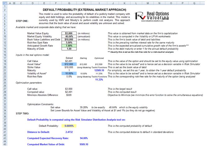
Figure 92.1: Default probability model setup
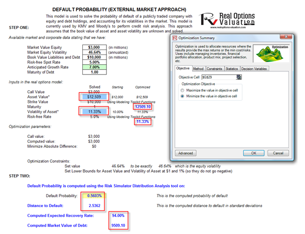
Figure 92.2: Default probability of a publicly traded entity
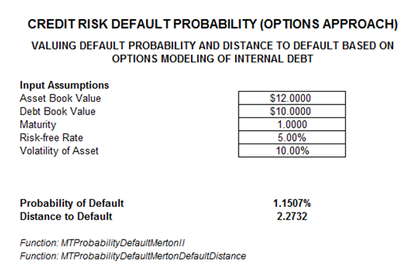
Figure 92.3: Default probability of a privately held entity
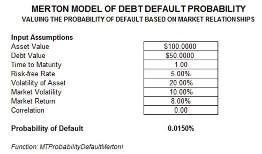
Figure 92.4: Default probability of a privately held entity calibrated to market fluctuations
Empirical Models of Probability of Default
As mentioned, empirical models of the probability of default are used to compute an individual’s default probability, applicable within the retail banking arena, where empirical or actual historical or comparable data exist on past credit defaults. The dataset in Figure 92.5 represents a sample of several thousand previous loans, credit, or debt issues. The data show whether each loan had defaulted or not (0 for no default, and 1 for default) as well as the specifics of each loan applicant’s age, education level (1 to 3 indicating high school, university, or graduate professional education), years with current employer, and so forth. The idea is to model these empirical data to see which variables affect the default behavior of individuals, using Risk Simulator’s Maximum Likelihood Model. The resulting model will help the bank or credit issuer compute the expected probability of default of an individual credit holder having specific characteristics.
Illustrative Example on Applying Empirical Models of Probability of Default
The example file is Probability of Default – Empirical and can be accessed through Modeling Toolkit | Prob of Default | Empirical (Individuals). To run the analysis, select the data on the left or any other dataset (include the headers) and make sure that the data have the same length for all variables, without any missing or invalid data. Then, using Risk Simulator, click on Risk Simulator | Forecasting | Maximum Likelihood Models. A sample set of results is provided in the MLE worksheet, complete with detailed instructions on how to compute the expected probability of default of an individual.
The Maximum Likelihood Estimates (MLE) approach on a binary multivariate logistic analysis is used to model dependent variables to determine the expected probability of success of belonging to a certain group. For instance, given a set of independent variables (e.g., age, income, education level of credit card or mortgage loan holders), we can model the probability of default using MLE. A typical regression model is invalid because the errors are heteroskedastic and non-normal, and the resulting estimated probability estimates will sometimes be above 1 or below 0. MLE analysis handles these problems using an iterative optimization routine. The computed results show the coefficients of the estimated MLE intercept and slopes.¹
The coefficients estimated are actually the logarithmic odds ratios and cannot be interpreted directly as probabilities. A quick but simple computation is first required. The approach is straightforward. To estimate the probability of success of belonging to a certain group (e.g., predicting if a debt holder will default given the amount of debt he holds), simply compute the estimated Y value using the MLE coefficients. Figure 92.6 illustrates an individual with 8 years at a current employer and current address, a low 3% debt to income ratio, and $2,000 in credit card debt has a log odds ratio of –3.1549. The inverse antilog of the odds ratio is obtained by computing: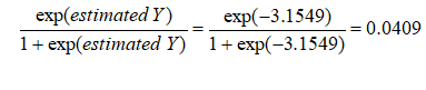
¹For instance, the coefficients are estimates of the true population β values in the following equation: Y = β0 + β1X1 + β2X2 + … + βnXn. The standard error measures how accurate the predicted coefficients are, and the Z-statistics are the ratios of each predicted coefficient to its standard error. The Z-statistic is used in hypothesis testing, where we set the null hypothesis (Ho) such that the real mean of the coefficient is equal to zero, and the alternate hypothesis (Ha) such that the real mean of the coefficient is not equal to zero. The Z-test is very important as it calculates if each of the coefficients is statistically significant in the presence of the other regressors. This means that the Z-test statistically verifies whether a regressor or independent variable should remain in the model or it should be dropped. That is, the smaller the p-value, the more significant the coefficient. The usual significant levels for the p-value are 0.01, 0.05, and 0.10, corresponding to the 99%, 95%, and 99% confidence levels.
So, such a person has a 4.09% chance of defaulting on the new debt. Using this probability of default, you can then use the Credit Analysis – Credit Premium model to determine the additional credit spread to charge this person given this default level and the customized cash flows anticipated from this debt holder.
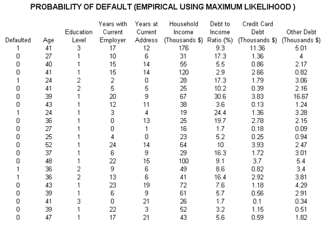
Figure 92.5: Empirical analysis of probability of default
The p-values are 0.01, 0.05, and 0.10, corresponding to the 99%, 95%, and 99% confidence levels.
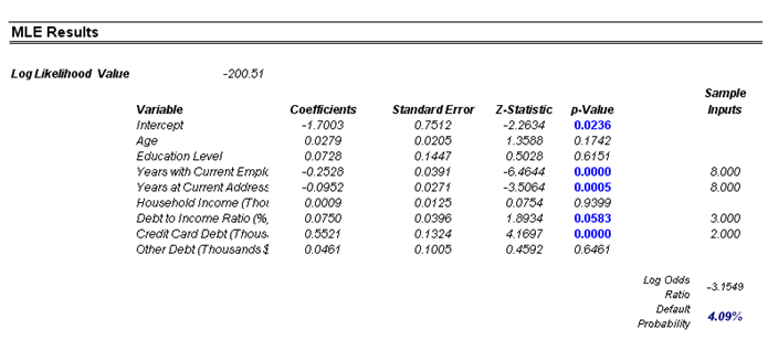
Figure 92.6: MLE results
Loss Given Default and Expected Losses
As shown previously, the probability of default is a key parameter for computing the credit risk of a portfolio. In fact, the Basel II/III Accord requires that the probability of default as well as other key parameters, such as the loss given default (LGD) and exposure at default (EAD), be reported as well. The reason is that a bank’s expected loss is equivalent to:
Expected Losses = (Probability of Default) × (Probability of Default) × (Exposure at Default)
or simply EL = PD × LGD × EAD.
PD and LGD are both percentages, whereas EAD is a value. As we have shown how to compute PD earlier, we will now revert to some estimations of LGD. There are several methods used to estimate LGD. The first is through a simple empirical approach where we set LGD = 1 – Recovery Rate. That is, whatever is not recovered at default is the loss at default, computed as the charge-off (net of recovery) divided by the outstanding balance:
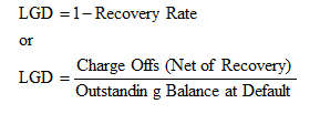
Therefore, if market data or historical information are available, LGD can be segmented by various market conditions, types of obligor, and other pertinent segmentations. LGD can then be readily read off a chart.
A second approach to estimate LGD is more attractive in that if the bank has available information, it can attempt to run some econometric models to create the best-fitting model under an ordinary least squares approach. By using this approach, a single model can be determined and calibrated, and this same model can be applied under various conditions, with no data mining required. However, in most econometric models, a normal transformation will have to be performed first. Supposing the bank has some historical LGD data (Figure 92.7), the best-fitting distribution can be found using Risk Simulator (select the historical data, click on Risk Simulator | Analytical Tools | Distributional Fitting (Single Variable) to perform the fitting routine). The result is a beta distribution for the thousands of LGD values.
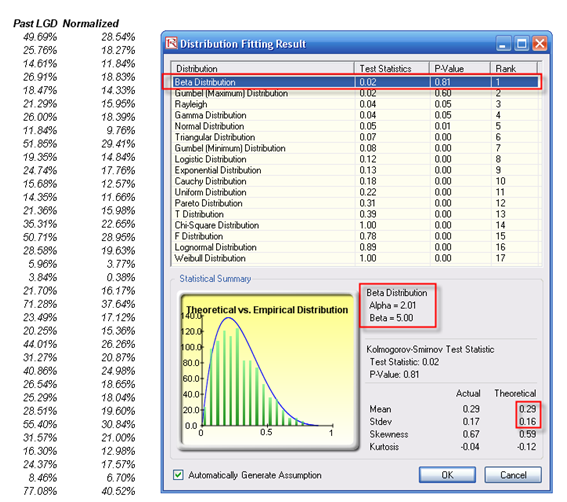
Figure 92.7: Fitting historical LGD data
Then, using the Distribution Analysis tool in Risk Simulator, obtain the theoretical mean and standard deviation of the fitted distribution (Figure 92.8). Then transform the LGD variable using the MTNormalTransform function in the Modeling Toolkit software. For instance, the value of 49.69% will be transformed and normalized to 28.54%. Using this newly transformed dataset, you can run some nonlinear econometric models to determine LGD.
For instance, a partial list of independent variables that might be significant for a bank, in terms of determining and forecast the LGD value, might include:
- Debt to capital ratio
- Profit margin
- Revenue
- Current assets to current liabilities
- Risk rating at default and one year before default
- Industry
- Authorized balance at default
- Collateral value
- Facility type
- Tightness of covenant
- Seniority of debt
- Operating income to sales ratio (and other efficiency ratios)
- Total asset, total net worth, total liabilities
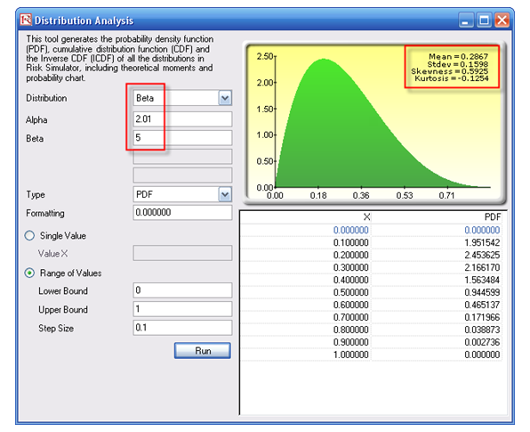
Figure 92.8: Distributional analysis tool
Economic Capital and Value at Risk
Economic capital is critical to a bank as it links a bank’s earnings and returns to risks that are specific to business lines or business opportunities. In addition, these economic capital measurements can be aggregated into a portfolio of holdings. Value at Risk (VaR) is used in trying to understand how the entire organization is affected by the various risks of each holding as aggregated into a portfolio, after accounting for cross-correlations among various holdings. VaR measures the maximum possible loss given some predefined probability level (e.g., 99.90%) over some holding period or time horizon (e.g., 10 days). Senior management at the bank usually selects the probability or confidence interval, which is typically a decision made by senior management at the bank and reflects the board’s risk appetite. Stated another way, we can define the probability level as the bank’s desired probability of surviving per year. In addition, the holding period is usually chosen such that it coincides with the time period it takes to liquidate a loss position.
VaR can be computed in several ways. Two main families of approaches exist: structural closed-form models and Monte Carlo risk simulation approaches. We showcase both methods in this chapter, starting with the structural models.
The second and much more powerful approach is Monte Carlo risk simulation. Instead of simply correlating individual business lines or assets, entire probability distributions can be correlated using mathematical copulas and simulation algorithms, by using Risk Simulator. In addition, tens to hundreds of thousands of scenarios can be generated using simulation, providing a very powerful stress-testing mechanism for valuing VaR. Distributional fitting methods are applied to reduce the thousands of data points into their appropriate probability distributions, allowing their modeling to be handled with greater ease.
Illustrative Example: Structural VaR Models
This first VaR example model used is Value at Risk – Static Covariance Method, accessible through Modeling Toolkit | Value at Risk | Static Covariance Method. This model is used to compute the portfolio’s VaR at a given percentile for a specific holding period, after accounting for the cross-correlation effects between the assets (Figure 92.9). The daily volatility is the annualized volatility divided by the square root of trading days per year. Typically, positive correlations tend to carry a higher VaR compared to zero correlation asset mixes, whereas negative correlations reduce the total risk of the portfolio through the diversification effect (Figures 92.9 and 92.10). The approach used is a portfolio VaR with correlated inputs, where the portfolio has multiple asset holdings with different amounts and volatilities. Each asset is also correlated to each other. The covariance or correlation structural model is used to compute the VaR given a holding period or horizon and percentile value (typically 10 days at 99% confidence). Of course, the example illustrates only a few assets or business lines or credit lines for simplicity’s sake. Nonetheless, using the VaR function (MTVaRCorrelationMethod) in the Modeling Toolkit, many more lines, assets, or businesses can be modeled.
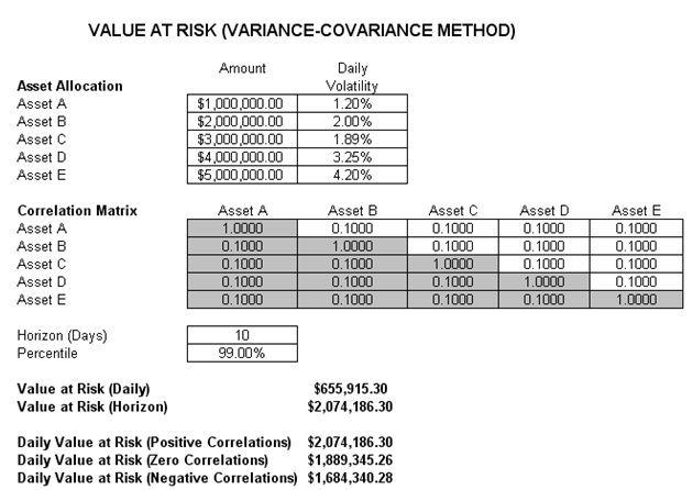
Figure 92.9: Computing Value at Risk using the structural covariance method
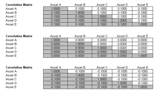
Figure 92.10: Different correlation levels
Illustrative Example: VaR Models Using Monte Carlo Risk Simulation
The model used is Value at Risk – Portfolio Operational and Credit Risk VaR Capital Adequacy and is accessible through Modeling Toolkit | Value at Risk | Portfolio Operational and Credit Risk VaR Capital Adequacy. This model shows how operational risk and credit risk parameters are fitted to statistical distributions and their resulting distributions are modeled in a portfolio of liabilities to determine the VaR (99.50th percentile certainty) for the capital requirement under Basel II/III requirements. It is assumed that the historical data of the operational risk impacts (Historical Data worksheet) are obtained through econometric modeling of the Key Risk Indicators.
The Distributional Fitting Report worksheet is a result of running a distributional fitting routine in Risk Simulator to obtain the appropriate distribution for the operational risk parameter. Using the resulting distributional parameter, we model each liability’s capital requirements within an entire portfolio. Correlations can also be inputted if required, between pairs of liabilities or business units. The resulting Monte Carlo simulation results show the VaR capital requirements.
Note that an appropriate empirically based historical VaR cannot be obtained if distributional fitting and risk-based simulations were not first run. The VaR will be obtained only by running simulations. To perform distributional fitting, follow these steps:
- In the Historical Data worksheet (Figure 92.11), select the data area (cells C5:L104) and click on Risk Simulator | Analytical Tools | Distributional Fitting (Single Variable).
- Browse through the fitted distributions and select the best-fitting distribution (in this case, the exponential distribution in Figure 92.12) and click OK.
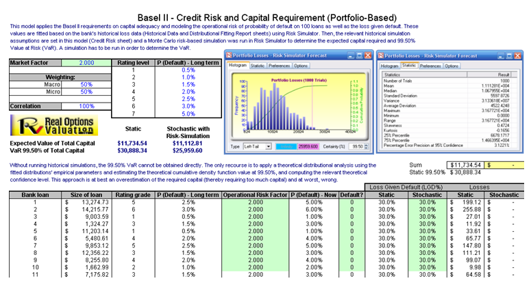
Figure 92.11: Sample historical bank loans
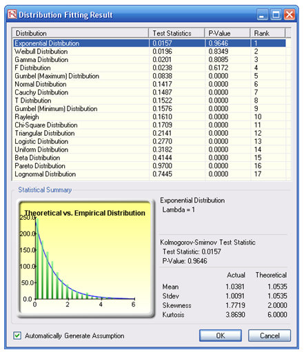
Figure 92.12: Data fitting results
- You may now set the assumptions on the Operational Risk Factors with the exponential distribution (fitted results show Lambda = 1) in the Credit Risk Note that the assumptions have already been set for you in advance. You may set the assumption by going to cell F27 and clicking on Risk Simulator | Set Input Assumption, selecting Exponential distribution and entering 1 for the Lambda value, and clicking OK. Continue this process for the remaining cells in column F, or simply perform a Risk Simulator Copy and Risk Simulator Paste on the remaining cells.
- Note that since the cells in column F have assumptions set, you will first have to clear them if you wish to reset and copy/paste parameters. You can do so by first selecting cells F28:F126 and clicking on the Remove Parameter icon or select Risk Simulator | Remove Parameter.
- Then select cell F27, click on the Risk Simulator Copy icon or select Risk Simulator | Copy Parameter, and then select cells F28:F126 and click on the Risk Simulator Paste icon or select Risk Simulator | Paste Parameter.
- Next, you can get assumptions that can be set such as the probability of default using the Bernoulli Distribution (column H) and Loss Given Default (column J). Repeat the procedure in Step 3 if you wish to reset the assumptions.
- Run the simulation by clicking on the RUN icon or clicking on Risk Simulator | Run Simulation.
- Obtain the Value at Risk by going to the forecast chart once the simulation is done running and selecting Left-Tail and typing in 50. Hit TAB on the keyboard to enter the confidence value and obtain the VaR of $25,959 (Figure 92.13).
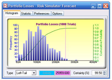
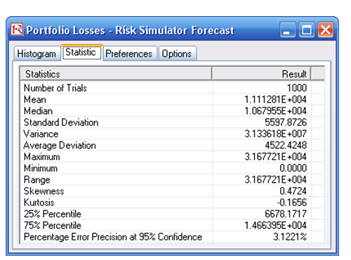
Figure 92.13: Simulated forecast results and the 99.50% Value at Risk value
Another example on VaR computation is shown next, where the model Value at Risk – Right Tail Capital Requirements is used, available through Modeling Toolkit | Value at Risk | Right Tail Capital Requirements.
This model shows the capital requirements per Basel II/III requirements (99.95th percentile capital adequacy based on a specific holding period’s VaR). Without running risk-based historical and Monte Carlo simulation using Risk Simulator, the required capital is $37.01M (Figure 92.14) as compared to only $14.00M that is required using a correlated simulation (Figure 92.15). This is due to the cross-correlations between assets and business lines and can only be modeled only using Risk Simulator. This lower VaR is preferred as banks can be required to hold less required capital and can reinvest the remaining capital in various profitable ventures, thereby generating higher profits.
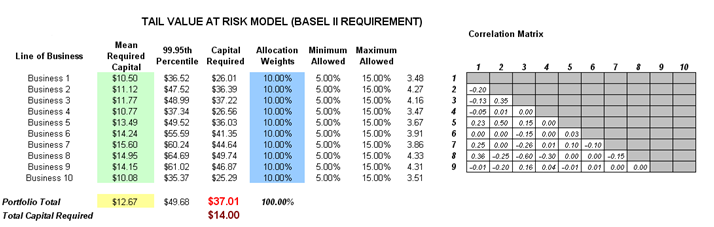
Figure 92.14: Right-tail VaR model
To run the model, follow these steps:
- Click on Risk Simulator | Run Simulation. If you had other models open, make sure you first click on Risk Simulator | Change Profile, and select the Tail VaR profile before starting.
- When the simulation is complete, select Left-Tail in the forecast chart and enter in 95 in the Certainty box, and hit TAB on the keyboard to obtain the value of $14.00M Value at Risk for this correlated simulation.
- Note that the assumptions have already been set for you in advance in the model in cells C6:C15. However, you may set them again by going to cell C6 and clicking on Risk Simulator | Set Input Assumption, selecting your distribution of choice or using the default Normal Distribution or performing a distributional fitting on historical data, then clicking OK. Continue this process for the remaining cells in column C. You may also decide to first Remove Parameters of these cells in column C and setting your own distributions. Further, correlations can be set manually when assumptions are set (Figure 92.16) or by going to Risk Simulator | Edit Correlations (Figure 92.17) after all the assumptions are set.
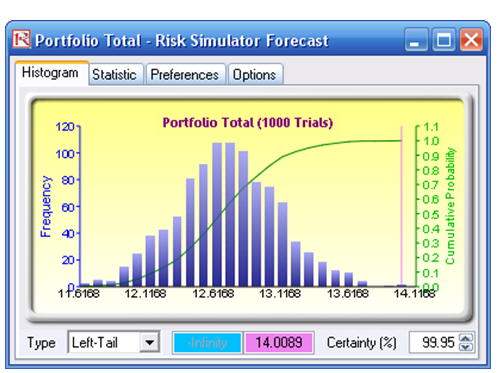
Figure 92.15: Simulated results of the portfolio VaR
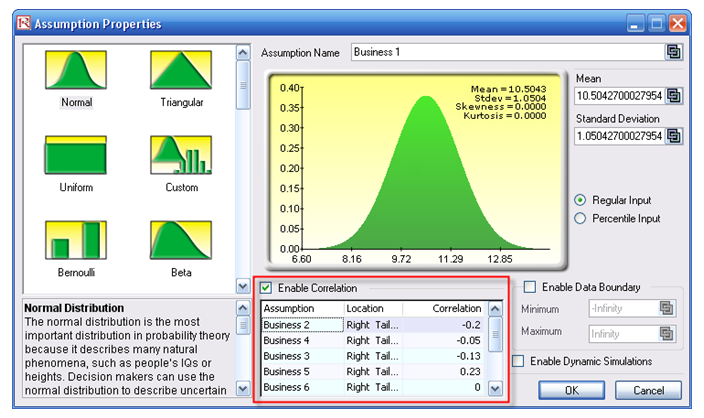
Figure 92.16: Setting correlations one at a time
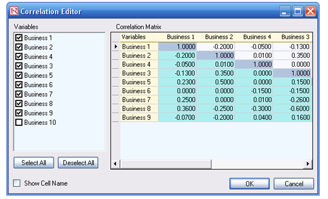
Figure 92.17: Setting correlations using the correlation matrix routine
If risk simulation was not run, the VaR or economic capital required would have been $37M, as opposed to only $14M. All cross-correlations between business lines have been modeled, as are stress and scenario tests, and thousands and thousands of possible iterations are run. Individual risks are now aggregated into a cumulative portfolio level VaR.
Efficient Portfolio Allocation and Economic Capital VaR
As a side note, by performing portfolio optimization, a portfolio’s VaR actually can be reduced. We start by first introducing the concept of stochastic portfolio optimization through an illustrative hands-on example. Then, using this portfolio optimization technique, we apply it to four business lines or assets to compute the VaR or an un-optimized versus an optimized portfolio of assets, and see the difference in computed VaR. You will note that in the end, the optimized portfolio bears less risk and has a lower required economic capital.
Illustrative Example: Stochastic Portfolio Optimization
The optimization model used to illustrate the concepts of stochastic portfolio optimization is Optimization – Stochastic Portfolio Allocation and can be accessed via Modeling Toolkit | Optimization | Stochastic Portfolio Allocation. This model shows four asset classes with different risk and return characteristics. The idea here is to find the best portfolio allocation such that the portfolio’s bang for the buck or returns to risk ratio, is maximized. That is, in order to allocate 100% of an individual’s investment among several different asset classes (e.g., different types of mutual funds or investment styles: growth, value, aggressive growth, income, global, index, contrarian, momentum, etc.), an optimization is used. This model is different from others in that there exist several simulation assumptions (risk and return values for each asset), as seen in Figure 92.18.
In other words, a simulation is first run, then optimization is executed, and the entire process is repeated multiple times to obtain distributions of each decision variable. The entire analysis can be automated using Stochastic Optimization.
In order to run an optimization, several key specifications on the model have to be identified first:
Objective: Maximize Return to Risk Ratio (C12)
Decision Variables: Allocation Weights (E6:E9)
Restrictions on Decision Variables: Minimum and Maximum Required (F6:G9)
Constraints: Portfolio Total Allocation Weights 100% (E11 is set to 100%)
Simulation Assumptions: Return and Risk Values (C6:D9)
The model shows the various asset classes. Each asset class has its own set of annualized returns and annualized volatilities. These return and risk measures are annualized values such that they can be compared consistently across different asset classes. Returns are computed using the geometric average of the relative returns, while the risks are computed using the logarithmic relative stock returns approach.
Column E, Allocation Weights, holds the decision variables, which are the variables that need to be tweaked and tested such that the total weight is constrained at 100% (cell E11). Typically, to start the optimization, we will set these cells to a uniform value, where in this case, cells E6 to E9 are set at 25% each. In addition, each decision variable may have specific restrictions in its allowed range. In this example, the lower and upper allocations allowed are 10% and 40%, as seen in columns F and G. This setting means that each asset class can have its own allocation boundaries.
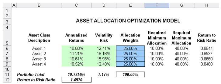
Figure 92.18: Asset allocation model ready for stochastic optimization
Column H shows the return to risk ratio, which is simply the return percentage divided by the risk percentage, where the higher this value, the higher the bang for the buck. The remaining sections of the model show the individual asset class rankings by returns, risk, return to risk ratio, and allocation. In other words, these rankings show at a glance which asset class has the lowest risk, or the highest return, and so forth.
Running an Optimization
To run this model, simply click on Risk Simulator | Optimization | Run Optimization. Alternatively, and for practice, you can set up the model using the following approach:
- Start a new profile(Risk Simulator | New Profile).
- For stochastic optimization, set distributional assumptions on the risk and returns for each asset That is, select cell C6 and set an assumption (Risk Simulator | Set Input Assumption), and make your own assumption as required. Repeat for cells C7 to D9.
- Select cell E6 and define the decision variable (Risk Simulator | Optimization | Decision Variables or click on the Define Decision icon) and make it a Continuous Variable and then link the decision variable’s name and minimum/maximum required to the relevant cells (B6, F6, G6).
- Then use the Risk Simulator Copy on cell E6, select cells E7 to E9, and use Risk Simulator’s Paste (Risk Simulator | Copy Parameter and Risk Simulator | Paste Parameter or use the Risk Simulator copy and paste icons). Make sure you do not use Excel’s regular copy and paste functions.
- Next, set up the optimization’s constraints by selecting Risk Simulator | Optimization | Constraints, selecting ADD, and selecting the cell E11, and making it equal 100% (total allocation, and do not forget the % sign).
- Select cell C12, the objective to be maximized and make it the objective: Risk Simulator | Optimization | Set Objective or click on the O icon.
- Run the simulation by going to Risk Simulator | Optimization | Run Optimization. Review the different tabs to make sure that all the required inputs in steps 2 and 3 are correct. Select Stochastic Optimization and let it run for 500 trials repeated 20 times (Figure 92.19 illustrates these setup steps).
You may also try other optimization routines where:
Static Optimization is an optimization that is run on a static model, where no simulations are run. This optimization type is applicable when the model is assumed to be known and no uncertainties exist. Also, a static optimization can be run first to determine the optimal portfolio and its corresponding optimal allocation of decision variables before more advanced optimization procedures are applied. For instance, before running a stochastic optimization problem, a static optimization is run first to determine if there exist solutions to the optimization problem before a more protracted analysis is performed.
Dynamic Optimization is applied when Monte Carlo simulation is used together with optimization. Another name for such a procedure is Simulation-Optimization. In other words, a simulation is run for N trials, and then an optimization process is run for M iterations until the optimal results are obtained, or an infeasible set is found. That is, using Risk Simulator’s Optimization module, you can choose which forecast and assumption statistics to use and replace in the model after the simulation is run. Then, these forecast statistics can be applied in the optimization process. This approach is useful when you have a large model with many interacting assumptions and forecasts, and when some of the forecast statistics are required in the optimization.
Stochastic Optimization is similar to the dynamic optimization procedure except that the entire dynamic optimization process is repeated T times. The results will be a forecast chart of each decision variable with T values. In other words, a simulation is run and the forecast or assumption statistics are used in the optimization model to find the optimal allocation of decision variables. Then another simulation is run, generating different forecast statistics, and these new updated values are then optimized, and so forth. Hence, each of the final decision variables will have its own forecast chart, indicating the range of the optimal decision variables. For instance, instead of obtaining single-point estimates in the dynamic optimization procedure, you can now obtain a distribution of the decision variables, and, hence, a range of optimal values for each decision variable, also known as stochastic optimization.
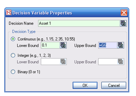
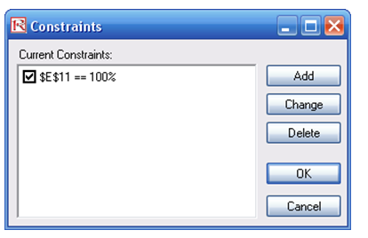
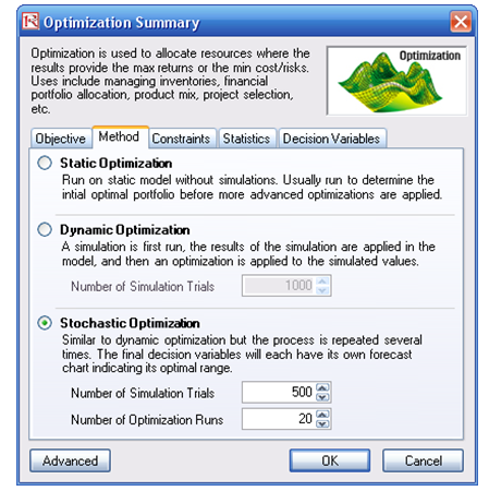
Figure 92.19: Setting up the stochastic optimization problem
Viewing and Interpreting Forecast Results
Stochastic optimization is performed when a simulation is first run and then the optimization is run. Then the whole analysis is repeated multiple times. The result is a distribution of each decision variable, rather than a single-point estimate (Figure 92.20). This means that instead of saying you should invest 30.57% in Asset 1, the optimal decision is to invest between 30.10% and 30.99% as long as the total portfolio sums to 100%. This way the optimization results provide management or decision makers a range of flexibility in the optimal decisions. Refer to Chapter 11 of Modeling Risk: Applying Monte Carlo Simulation, Real Options Analysis, Forecasting, and Optimization by Dr. Johnathan Mun for more detailed explanations about this model, the different optimization techniques, and an interpretation of the results. Chapter 11’s appendix also details how the risk and return values are computed.
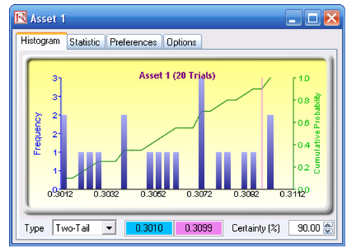
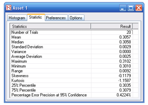
Figure 92.20: Simulated results from the stochastic optimization approach
Illustrative Example: Portfolio Optimization and Portfolio VaR
Now that we understand the concepts of optimized portfolios, let us see what the effects are on computed economic capital through the use of a correlated portfolio VaR. This model uses Monte Carlo simulation and optimization routines in Risk Simulator to minimize the Value at Risk of a portfolio of assets (Figure 92.21). The file used is Value at Risk – Optimized and Simulated Portfolio VaR, which is accessible via Modeling Toolkit | Value at Risk | Optimized and Simulated Portfolio VaR. In this example, we intentionally used only four asset classes to illustrate the effects of an optimized portfolio. In real life, we can extend this to cover a multitude of asset classes and business lines. Here we illustrate the use of a left-tail VaR, as opposed to a right-tail VaR, but the concepts are similar.
First, simulation is used to determine the 90% left-tail VaR. The 90% left-tail probability means that there is a 10% chance that losses will exceed this VaR for a specified holding period. With an equal allocation of 25% across the four asset classes, the VaR is determined using simulation (Figure 92.21). The annualized returns are uncertain and hence simulated. The VaR is then read off the forecast chart. Then optimization is run to find the best portfolio subject to the 100% allocation across the four projects that will maximize the portfolio’s bang for the buck (returns to risk ratio). The resulting optimized portfolio is then simulated once again, and the new VaR is obtained (Figure 92.22). The VaR of this optimized portfolio is a lot less than the not-optimized portfolio.
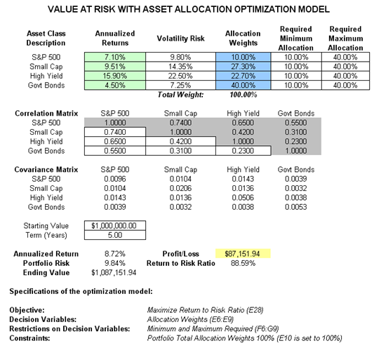
Figure 92.21: Computing Value at Risk (VaR) with simulation
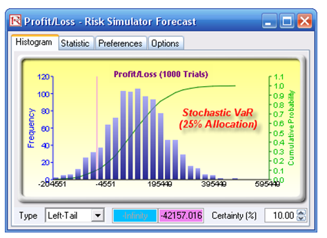
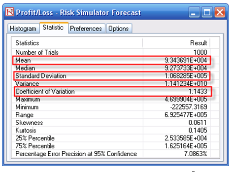
Figure 92.22: Non-optimized Value at Risk
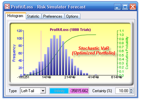
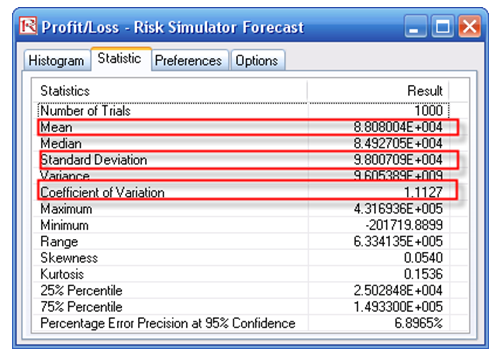
Figure 92.23: Optimal portfolio’s Value at Risk through optimization and simulation
Hurdle Rates and Required Rate of Return
Another related item in the discussion of risk in the context of Basel II/III Accords is the issue of hurdle rates, or the required rate of return on investment that is sufficient to justify the amount of risk undertaken in the portfolio. There is a nice theoretical connection between uncertainty and volatility whereby the discount rate of a specific risk portfolio can be obtained. In a financial model, the old axiom of high risk, high return is seen through the use of a discount rate. That is, the higher the risk of a project, the higher the discount rate should be to risk-adjust this riskier project so that all projects are comparable.
There are two methods for computing the hurdle rate. The first is an internal model, where the VaR of the portfolio is computed first. This economic capital is then compared to the market risk premium. That is, we have
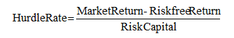
That is, assuming that a similar set of comparable investments are obtained in the market, based on tradable assets, the market return is obtained. Using the bank’s internal cash flow models, all future cash flows can be discounted at the risk-free rate in order to determine the risk-free return. Finally, the difference is then divided into the VaR risk capital to determine the required hurdle rate. This concept is very similar to the capital asset pricing model (CAPM), which often is used to compute the appropriate discount rate for a discounted cash flow model (weighted average cost of capital, hurdle rates, multiple asset pricing models, and arbitrage pricing models are the other alternatives but are based on similar principles). The second approach is the use of the CAPM to determine the hurdle rate.