CONTINUED LIST OF ANALYTICAL METHODSSkywalk Digital2021-12-16T13:45:54+00:00
- Partial Correlations (Using Correlation Matrix). Runs and computes the Partial Correlation Matrix using your existing N × N full correlation matrix.
- Short Tip: Computes the Partial Correlation Matrix using an existing N × N full square correlation matrix.
- Model Input: Data Type C. Two or more input variables are required. Different variables are arranged in columns and all variables must have at least 2 data points each, with the same number of total data points or rows per variable. The total number of variables must match the number of rows, i.e., the data entered should be in an N × N matrix.
- Partial Correlations (Using Raw Data). Runs and computes the Partial Correlation Matrix using raw data of multiple columns.
- Short Tip: Computes the Partial Correlation Matrix using raw data.
- Model Input: Data Type C. Two or more input variables are required. Different variables are arranged in columns and all variables must have at least 5 data points each, with the same number of total data points or rows per variable.
-
-
-
- Principal Component Analysis. Principal component analysis, or PCA, makes multivariate data easier to model and summarize. To understand PCA, suppose we start with N variables that are unlikely to be independent of one another, such that changing the value of one variable will change another variable. PCA modeling will replace the original N variables with a new set of M variables that are less than N but are uncorrelated to one another, while at the same time, each of these M variables is a linear combination of the original N variables so that most of the variation can be accounted for just using fewer explanatory variables.
- Short Tip: Runs a principal component analysis on multiple variables.
- Model Input: Data Type C. Three or more input variables are required. Different variables are arranged in columns and all variables must have at least 5 data points each, with the same number of total data points or rows per variable.
-
-
- Process Capability. Given the user inputs of the process mean, sigma, as well as upper and lower specification limits, the model returns the various process capability measures (CP, CPK, PP), defective proportion units (DPU), defects per million opportunities (DPMO), output yield (%), and overall process sigma.
- Short Tip: Process capability is used to calculate projected manufacturing process output yield and defects.
- Model Input: Data Type A. Process Mean, Process Sigma, Upper Specification Limit USL, Lower Specification Limit LSL
-
-
-
- >2.2500
- >0.0500
- >2.1375
- >2.8125
- Quick Statistic. Absolute Values (ABS), Average (AVG), Count, Difference, LAG, Lead, LN, LOG, Max, Median, Min, Mode, Power, Rank Ascending, Rank Descending, Relative LN Returns, Relative Returns, Semi-Standard Deviation (Lower), Semi-Standard Deviation (Upper), Standard Deviation Population, Standard Deviation Sample, Sum, Variance (Population), Variance (Sample). Various basic statistics such as average, standard deviation, ranking, sum, and others are computed using a single variable dataset.
- Short Tip: Runs various basic statistics such as average, standard deviation, ranking, sum, etc.
- Model Input: Data Type A. One input variable is required with at least 3 data points or rows of data.
-
-
-
- ROC Curves, AUC, and Classification Tables. Runs the ROC and Classification Tables for numbers of failures and successes. The area under the curve (AUC) is computed using rectangular mode (R) and trapezoidal mode (T).
- Short Tip: Runs ROC and Classification tables for failures and successes and computes the area under the curve (AUC).
- Model Input: Data Type B. Two input variables are required: Failures and Successes, with at least 3 rows of data for each variable. Each variable needs to have the same number of data rows. A final input required is the Cutoff value.
- Failures, Successes, Cutoff:
-
-
-
- Seasonality. Many time-series data exhibit seasonality where certain events repeat themselves after some time period or seasonality period (e.g., ski resorts’ revenues are higher in winter than in summer, and this cycle will repeat itself every winter). The method tests for multiple periods of seasonalities (number of periods in one seasonal cycle).
- Short Tip: Runs various seasonality models to determine the best seasonality fit.
- Model Input: Data Type A. One input variable is required with at least 3 data points or rows of data and the maximum seasonality to test.
-
-
-
- Segmentation Clustering. Taking the original dataset, we run some internal algorithms (a combination of k-means hierarchical clustering and other methods-of-moments in order to find the best-fitting groups or natural statistical clusters) to statistically divide or segment the original dataset into multiple groups.
- Short Tip: Runs segmentation clustering of an existing dataset and segregates the data into various statistical groups.
- Model Input: Data Type A. One input variable is required with at least 3 data points or rows of data.
-
-
-
- Skew and Kurtosis: Shapiro–Wilk and D’Agostino–Pearson. Runs the Skew and Kurtosis tests to see if the data has both statistics equal to zero (normality), and the D’Agostino–Pearson test if skew and kurtosis are simultaneously zero. The null hypothesis is the data has zero skew and kurtosis, approximating normality.
- Short Tip: Tests if both skew and kurtosis are equal to zero and therefore approximating normality (H0: skew and kurtosis are zero and data approximates normality).
- Model Input: Data Type A. One input variable is required with at least 5 rows of data.
-
-
-
- Specifications Cubed Test (Ramsey’s RESET). Ramsey’s regression specification error test (RESET) looks for general misspecification of your model using an F-Test variation and cubed predictions. Rejecting the null hypothesis indicates some sort of misspecification in the model. The null hypothesis tested is that the current model is correctly specified.
- Short Tip: Ramsey’s regression specification error test (RESET) looks for general misspecification of your model using an F-Test variation and cubed predictions.
- Model Input: Data Type C. One dependent variable and one or more independent variables with custom modifications.
-
-
-
- >VAR1
- >VAR2; LN(VAR3); (VAR4)^2
- Specifications Squared Test (Ramsey’s RESET). Ramsey’s regression specification error test (RESET) looks for general misspecification of your model using an F-Test variation and squared predictions. Rejecting the null hypothesis indicates some sort of misspecification in the model. The null hypothesis tested is that the current model is correctly specified.
- Short Tip: Ramsey’s regression specification error test (RESET) looks for general misspecification of your model using an F-Test variation and squared predictions.
- Model Input: Data Type C. One dependent variable and one or more independent variables with custom modifications.
-
-
-
- >VAR1
- >VAR2; LN(VAR3); (VAR4)^2
- Stationarity: Augmented Dickey–Fuller. Runs the unit root test for stationarity with no constant intercept and no linear trend using a multi-order autoregressive AR(p) process. The null hypothesis tested is that there is a unit root, and the time series is not stationary.
- Short Tip: Unit root test with a constant and trend (H0: data exhibit unit root and the time series is a nonstationary AR(p) series).
- Model Input: Data Type A. One input variable is required with at least 10 rows of data.
-
-
-
- Stationarity: Dickey–Fuller (Constant and Trend). Runs the unit root test for stationarity with a constant intercept and a linear trend using a first-order autoregressive AR(1) process. The null hypothesis tested is that there is a unit root, and the time series is not stationary.
- Short Tip: Unit root test with constant and trend (H0: data exhibit unit root and the time series is a nonstationary AR(1) series).
- Model Input: Data Type A. One input variable is required with at least 10 rows of data.
-
-
-
- Stationarity: Dickey–Fuller (Constant No Trend). Runs the unit root test for stationarity with a constant intercept and no linear trend using a first-order autoregressive AR(1) process. The null hypothesis tested is that there is a unit root, and the time series is not stationary.
- Short Tip: Unit root test with a constant but no trend (H0: data exhibit unit root and the time series is a nonstationary AR(1) series).
- Model Input: Data Type A. One input variable is required with at least 10 rows of data.
-
-
-
- Stationarity: Dickey–Fuller (No Constant No Trend). Runs the unit root test for stationarity with no constant intercept and no linear trend using a first-order autoregressive AR(1) process. The null hypothesis tested is that there is a unit root, and the time series is not stationary.
- Short Tip: Unit root test without constant or trend (H0: data exhibit unit root and the time series is a nonstationary AR(1) series).
- Model Input: Data Type A. One input variable is required with at least 10 rows of data.
-
-
-
- Stepwise Regression.
- Short Tip: Runs various multiple stepwise linear regression
- Model Input: Data Type C. Two sets of variables are required: One Dependent Variable and One or Multiple Independent Variables, with at least 5 rows of data in each variable, with the same number of total data points or rows per variable.
- Dependent Variable, Independent Variables:
-
-
-
-
- Stepwise Regression(Backward). In the backward method, we run a regression with Y on all X variables and, reviewing each variable’s p-value, systematically eliminate the variable with the largest p-value. Then run a regression again, repeating each time until all p-values are statistically significant.
- Stepwise Regression(Correlation). In the correlation method, the dependent variable Y is correlated to all the independent variables X, and starting with the X variable with the highest absolute correlation value, a regression is run. Then subsequent X variables are added until the p-values indicate that the new X variable is no longer statistically significant. This approach is quick and simple but does not account for interactions among variables, and an X variable, when added, will statistically overshadow other variables.
- Stepwise Regression(Forward). In the forward method, we first correlate Y with all X variables, run a regression for Y on the highest absolute value correlation of X, and obtain the fitting Then, correlate these errors with the remaining X variables and choose the highest absolute value correlation among this remaining set and run another regression. Repeat the process until the p-value for the latest X variable coefficient is no longer statistically significant and then stop the process.
- Stepwise Regression(Forward-Backward). In the forward and backward method, apply the forward method to obtain three X variables, and then apply the backward approach to see if one of them needs to be eliminated because it is statistically insignificant. Repeat the forward method and then the backward method until all remaining X variables are considered.
- Stochastic Process. Sometimes variables cannot be readily predicted using traditional means, and these variables are said to be stochastic. Nonetheless, most financial, economic, and naturally occurring phenomena (e.g., the motion of molecules through the air) follow a known mathematical law or relationship. Although the resulting values are uncertain, the underlying mathematical structure is known and can be simulated using Monte Carlo risk simulation.
- Short Tip: Generates various time-series stochastic process
- Model Input: Data Type A. Multiple manual inputs are required. The specific input requirements depend on the stochastic process selected.
- Initial Value, Drift Rate, Volatility, Horizon, Steps, Random Seed, Iterations
-
-
-
- >100
- >0.05
- >0.25
- >10
- >100
- >123456
-
- Brownian Motion Random Walk Process. The Brownian motion random walk process takes the form of
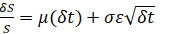 for regular options simulation, or a more generic version takes the form of
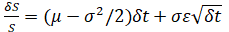 for a geometric For an exponential version, we simply take the exponentials, and, as an example, we have ,
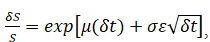 where we define S as the variable’s previous value, δS as the change in the variable’s value from one step to the next, μ as the annualized growth or drift rate, and σ as the annualized volatility
- Mean-Reversion Process. The following describes the mathematical structure of a mean-reverting process with drift:
 . Here we define η as the rate of reversion to the mean and
 as the long-term value that the process reverts to.
- Jump-Diffusion Process. A jump-diffusion process is like a random walk process but includes a probability of a jump at any point in time. The occurrences of such jumps are completely random, but their probability and magnitude are governed by the process itself. We have the structure
 for a jump diffusion process, and we define θ as the jump size of S, F(λ) as the inverse of the Poisson cumulative probability distribution, and λ as the jump rate of S.
- Jump-Diffusion Process with Mean Reversion. This model is essentially a combination of all three models discussed above (geometric Brownian motion with mean-reversion process and a jump-diffusion process).
- Structural Break. Tests if the coefficients in different datasets are equal and are most commonly used in time-series analysis to test for the presence of a structural break. A time-series dataset can be divided into two subsets and each subset is tested on the other and on the entire dataset to statistically determine if, indeed, there is a break starting at a particular time period. A one-tailed hypothesis test is performed on the null hypothesis such that the two data subsets are statistically similar to one another; that is, there is no statistically significant structural break.
- Short Tip: Runs a structural break test at specified breakpoints using a dependent variable and one or more independent variables.
- Model Input: Data Type C. Two sets of variables are required: One Dependent Variable and One or Multiple Independent Variables, with at least 5 rows of data in each variable, with the same number of total data points or rows per variable.
- Dependent Variable, Independent Variables, Structural Break Points:
-
-
-
- >VAR1
- >VAR2; VAR3; …
- 6; 8
- Structural Equation Model: Path Estimation (Partial Least Squares). Structural Equation Model (SEM) is typically used to solve path-dependent structures with endogenous variables. In a standard multivariate regression, we have one dependent variable (Y) and multiple independent variables (Xi), where the latter are independent of each other. However, in situations where the independent variables are related (e.g., endogenous variables), then SEM is needed. For instance, if X3 is impacted by X1 and X2, and X4 is impacted by X1 and X3, these need to be modeled in a simultaneous structure and solved using partial least squares.
- Short Tip: Runs a Path Estimation model using sequential and simultaneous models (path analysis using Partial Least Squares method in Structural Equation Modeling).
- Model Input: Data Type C. One or Multiple Independent Variables, and One Dependent Variable, with at least 5 rows of data in each variable, with the same number of total data points or rows per variable.
- Independent Variables, Dependent Variable (repeat for all the paths, starting with the longest to the shortest, and make sure the last variable is the dependent variable)
-
-
-
- > VAR1; VAR2; VAR3; VAR4; VAR5
- > VAR1; VAR2; VAR3; VAR4
- > VAR1; VAR3; VAR4
- > VAR1; VAR2
- Survival and Hazard Tables (Kaplan–Meier). The Kaplan–Meier method, the most commonly used life-table method in medical practice, does permit comparisons between patient groups or between different therapies.
- Short Tip: Runs a Kaplan–Meier survival and hazard tables.
- Model Input: Data Type C. Three variables are required: Starting Points of Interval, At Risk at the End of Interval, Died at End of Interval, with at least 3 rows of data in each variable, with the same number of total data points or rows per variable.
- Starting Points of Interval, At Risk at the End of Interval, Died at End of Interval:
-
-
-
- Time-Series Analysis. In well-behaved time-series data (e.g., sales revenues and cost structures of large corporations), the values tend to have up to three elements: a base value, trend, and seasonality. Time-series analysis uses these historical data and decomposes them into these three elements and recomposes them into future forecasts. In other words, this forecasting method, like some of the others described, first performs a back fitting (backcast) of historical data before it provides estimates of future values (forecasts).
- Short Tip: Runs various time-series forecasts with optimization using historical data, accounting for history, trend, and seasonality, and selects the best-fitting model.
- Model Input: Data Type A. One input variable is required with at least 5 data points or rows of data, followed by simple manual inputs depending on the model selected:
-
-
-
-
- Time-Series Analysis (Auto). Selecting this automatic approach will allow the user to initiate an automated process in methodically selecting the best input parameters in each model and ranking the forecast models from best to worst by looking at their goodness-of-fit results and error measurements.
- Time-Series Analysis (DES). The double exponential-smoothing (DES) approach is used when the data exhibit a trend but no seasonality.
- Time-Series Analysis (DMA).The double moving average (DMA) method is used when the data exhibit a trend but no seasonality.
- Time-Series Analysis (HWA).The Holt–Winters Additive (HWA) approach is used when the data exhibit both seasonality and trend.
- Time-Series Analysis (HWM). The Holt–Winters Multiplicative (HWM) approach is used when the data exhibit both seasonality and trend.
- Time-Series Analysis (SA). The Seasonal Additive (SA) approach is used when the data exhibit seasonality but no trend.
- Time-Series Analysis (SM). The Seasonal Multiplicative (SM) approach is used when the data exhibit seasonality but no trend.
- Time-Series Analysis (SES). The Single Exponential Smoothing (SES) approach is used when the data exhibit no trend and no seasonality.
- Time-Series Analysis (SMA). The Single Moving Average (SMA) approach is used when the data exhibit no trend and no seasonality.
- Trending and Detrending. The typical methods for trending and detrending data are Difference, Exponential, Linear, Logarithmic, Moving Average, Polynomial, Power, Rate, Static Mean, and Static Median. This function detrends your original data to take out any trending components. In forecasting models, the process removes the effects of accumulating datasets from seasonality and trend to show only the absolute changes in values and to allow potential cyclical patterns to be identified after removing the general drift, tendency, twists, bends, and effects of seasonal cycles of a set of time-series For example, a detrended dataset may be necessary to discover a company’s true financial health—one may detrend increased sales around Christmas time to see a more accurate account of a company’s sales in a given year more clearly by shifting the entire dataset from a slope to a flat surface to better see the underlying cycles and fluctuations. The resulting charts show the effects of the detrended data against the original dataset, the percentage of the trend that was removed based on each detrending method employed, and the detrended dataset.
- Short Tip: Runs various time-series trend lines and forecasts using historical data, accounting for history, trend, and seasonality.
- Model Input: Data Type A. One input variable is required with at least 5 data points or rows of data, followed by simple manual inputs depending on the model selected:
-
-
-
- Value at Risk (VaR and CVaR). Given a return’s mean and standard deviation, as well as degrees of freedom, this model computes the Value at Risk (VaR) and Conditional Value at Risk (CVaR) of the returns using standardized normal and t distributions.
- Short Tip: Returns Value at Risk and Conditional Value at Risk based on distributions of returns using normal and t distributions.
- Model Input: Data Type A. Mean of Returns, Sigma of Returns, Degrees of Freedom
-
-
-
- Variances Homogeneity Bartlett’s Test. Returns the sample variance calculations for each of the input variables and using a pooled logarithmic Bartlett’s Test is applied. The null hypothesis tested is that the variances are homogeneous and statistically similar.
- Short Tip: Tests if the variances from various variables are similar (H0: all variances are equal or homogeneous).
- Model Input: Data Type C. Two or more input variables are required. Different variables are arranged in columns and all variables must have at least 3 data points each. Different numbers of total data points or rows per variable are allowed.
-
-
-
- Volatility: GARCH Models . The Generalized Autoregressive Conditional Heteroskedasticity model is used to model historical and forecast future volatility levels of a time series of raw price levels of a marketable security (e.g., stock prices, commodity prices, and oil prices). GARCH first converts the prices into relative returns, and then runs an internal optimization to fit the historical data to a mean-reverting volatility term structure, while assuming that the volatility is heteroskedastic in nature (changes over time according to some econometric characteristics). Several variations of this methodology are available in Risk Simulator, including EGARCH, EGARCH-T, GARCH-M, GJR-GARCH, GJR-GARCH-T, IGARCH, and T-GARCH. The dataset must be a time series of raw price levels.
- Short Tip: Generates various time-series volatility forecasts using GARCH model variations.
- Model Input: Data Type A. One data variable is required, followed by multiple manual inputs are required. The specific input requirements depend on the GARCH model selected.
- Stock Prices, Periodicity, Predictive Base, Forecast Periods, Variance Targeting, P, Q:
-
-
-
- >VAR1
- >250
- >12
- >12
- >1
- >1
- >1
- Volatility: Log Returns Approach. Calculates the volatility using the individual future cash flow estimates, comparable cash flow estimates, or historical prices, computing the annualized standard deviation of the corresponding logarithmic relative returns.
- Short Tip: Generates time-series volatility using the log-returns approach.
- Model Input: Data Type A. One data variable is required, followed by the periodicity (number of periods per season).
-
-
-
- Yield Curve (Bliss). Used for generating the term structure of interest rates and yield curve estimation with five beta and lambda estimated parameters. Some econometric modeling techniques are required to calibrate the values of several input parameters in this model. Virtually any yield curve shape can be interpolated using these models, which are widely used at banks around the world.
- Short Tip: Generates a time-series interest yield Bliss curve.
- Model Input: Data Type A. Multiple manual inputs are required.
- Beta 0, Beta 1, Beta 2, Lambda 1, Lambda 2, Starting Year, Ending Year, Step Size:
-
-
-
- >0.8
- >0.8
- >0.1
- >0.1
- >1.5
- >1
- >10
- >0.5
- >1
- Yield Curve (Nelson–Siegel). An interpolation model with four estimated parameters for generating the term structure of interest rates and yield curve Some econometric modeling techniques are required to calibrate the values of several input parameters in this model.
- Short Tip: Generates a time-series interest yield curve using the Nelson–Siegel method.
- Model Input: Data Type A. Multiple manual inputs are required.
- Beta 0, Beta 1, Beta 2, Lambda, Starting Year, Ending Year, Step Size:
-
-
-
- >0.03
- >0.04
- >0.02
- >0.25
- >1
- >15
- >1
error: Content is protected !!