To see which of the input assumptions drive total cost and schedule the most, a tornado analysis can be executed (Figure 2.3). Tornado analysis is a powerful analytical technique that captures the static impacts of each variable on the outcome of the model; that is, the tool automatically perturbs each variable in the model a preset amount, captures the fluctuation on the model’s forecast or final result, and lists the resulting perturbations ranked from the most significant to the least. Figure 2.3 illustrates the application of a tornado analysis, where Project D’s Expected Project Cost is selected as the target result to be analyzed. The target result’s precedents in the model are used in creating the tornado chart. Precedents are all the input and intermediate variables that affect the outcome of the model. For instance, if the model consists of A = B + C, and where C = D + E, then B, D, and E, are the precedents for A (C is not a precedent as it is only an intermediate calculated value). Figure 2.3 also shows the testing range of each precedent variable used to estimate the target result. If the precedent variables are simple inputs, then the testing range will be a simple perturbation based on the range chosen (e.g., the default is ±10%). Each precedent variable can be perturbed at different percentages if required (see the data grid at the bottom of the user interface). A wider range is important as it is better able to test extreme values rather than smaller perturbations around the expected values. In certain circumstances, extreme values may have a larger, smaller, or unbalanced impact (e.g., nonlinearities may occur where increasing or decreasing economies of scale and scope creep in for larger or smaller values of a variable) and only a wider range will capture this nonlinear impact.
The model can then be Monte Carlo risk simulated based on the minimum, most likely, and maximum values that were entered previously (Figure 2.2) and the results will show probability distributions of cost and schedule (Figure 2.4). For instance, the sample results show that for Project D, there is a 95% probability that the project can be completed at a cost of $398,742. The expected median or most likely value was originally $377,408 (Figure 2.2). With simulation, it shows that to be 95% sure that there are sufficient funds to complete the project, an additional buffer of $21,334 is warranted.
Note that the simulation chart in Figure 2.4 shows a trimodal distribution, i.e., there are three clusters and peaks in the histogram. This is because a probability of success on each task is set up in the model. See Chapter 6 for more details on how the overrun and probability of success works in the computations. Also refer to the appendices for more details on interpreting the distributional moments, simulation statistics, shape, and characteristics of distributions.¹
¹The results illustrated were obtained using the default example’s 1,000 simulation trials with a seed value of 123 for all Projects A through D, and simulations were set to run all projects simultaneously. In real-life projects, we recommend running 1,000–10,000 simulation trials depending on the complexity of the model.

Figure 2.2: Simple Linear Path Project Management with Cost and Schedule Risk
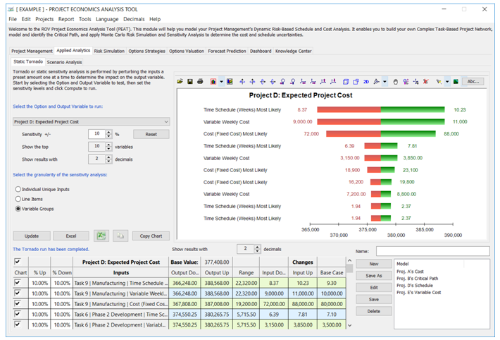
Figure 2.3: Simple Linear Path Tornado Analysis
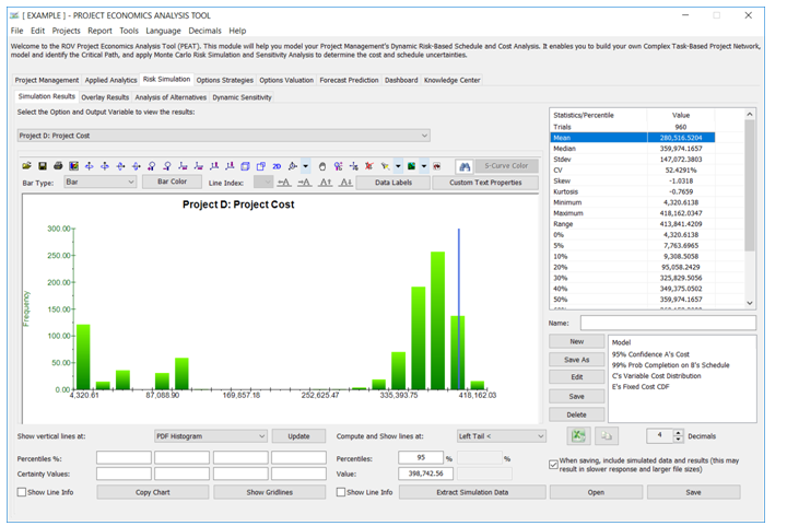
Figure 2.4: Monte Carlo Risk Simulated Results for Risky Cost and Schedule Values