File Name: Optimization – Optimizing Ordinary Least Squares
Location: Modeling Toolkit | Optimization | Optimizing Ordinary Least Squares
Brief Description: Illustrates how to solve a simple bivariate regression model with the ordinary least squares approach, using Risk Simulator’s optimization and its Regression Analysis tool
Requirements: Modeling Toolkit, Risk Simulator
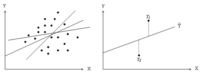
It is assumed that the user is sufficiently knowledgeable about the fundamentals of regression analysis. The general bivariate linear regression equation takes the form of Y = β0 + β1X + ε where β0 is the intercept, β1 is the slope, and ε is the error term. It is bivariate as there are only two variables, a Y or dependent variable, and an X or independent variable, where X is also known as the regressor (sometimes a bivariate regression is also known as a univariate regression as there is only a single independent variable X). The dependent variable is so named because it depends on the independent variable; for example, sales revenue depends on the amount of marketing costs expended on a product’s advertising and promotion, making the dependent variable sales and the independent variable marketing costs. An example of a bivariate regression is seen as simply inserting the best-fitting line through a set of data points in a two-dimensional plane as seen in the graphs shown next.
In other cases, a multivariate regression can be performed, where there are multiple or k number of independent X variables or regressors, where the general regression equation will now take the form:
![]()
However, fitting a line through a set of data points in a scatter plot, as shown in the graphs, may result in numerous possible lines. The best-fitting line is defined as the single unique line that minimizes the total vertical errors. That is, the sum of the absolute distances between the actual data points and the estimated line. To find the best-fitting unique line that minimizes the errors, a more sophisticated approach is applied, using regression analysis. Regression analysis, therefore, finds the unique best-fitting line by requiring that the total errors be minimized, or by calculating:![]() where
where![]() is the predicted value and Yi is the actual value.
is the predicted value and Yi is the actual value.
Only one unique line minimizes this sum of squared errors. The errors (vertical distances between the actual data and the predicted line) are squared to prevent the negative errors from canceling out the positive errors. Solving this minimization problem with respect to the slope and intercept requires calculating first derivatives and setting them equal to zero: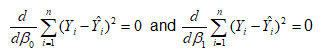
which yields the bivariate regression’s least squares equations: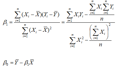
Model Background
In the model, we have a set of Y and X values, and we need to find the slope and intercept coefficients that minimize the sum of squared errors of the residuals, which will hence yield the ordinary least squares (OLS) unique line and regression equation. We start off with some initial inputs (say, 3000 for both the intercept and slope, where we will then attempt to find the correct answer, but we need to insert some values here as placeholders for now). Then we compute the predicted values using the initial slope and intercept, and then the residual error between the predicted and actual Y values (Figure 103.1). These residuals are then squared and summed to obtain the Sum of Squared Residuals. In order to get the unique line that minimizes the sum of the squared residual errors, we employ an optimization process, then compare the results to manually computed values, and then reconfirm the results using Risk Simulator’s Multiple Regression module.
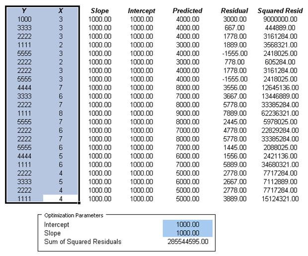
Figure 103.1: Optimizing ordinary least squares approach
Procedure
- Click on Risk Simulator | Change Profile and select OLS Optimization to open the preset profile.
- Go to the Model worksheet and click on Risk Simulator | Optimization | Run Optimization and click OK. To obtain a much higher level of precision, rerun the optimization a second time to make sure the solution converges. This is important as sometimes the starting points (the placeholder values of 3000) chosen are important and may require a second or third optimization run to converge to a solution.
If you wish to recreate the optimization, you can attempt to do so by following the instructions next. The optimization setup is also illustrated in Figure 103.2.
- Start a new profile(Risk Simulator | New Profile) and give it a name. Change the cells F37 and F38 back to some starting point, such as 3000 and 3000. This way, when the results are obtained, you see the new values.
- Select cell F39 and make it the Objective to minimize (this is the total sums of squares of the errors) by clicking on Risk Simulator | Optimization | Set Objective; then make sure F39 is selected and click Minimize.
- Set the decision variablesas the intercept and slope (cells F37 and F38, one at a time) by first selecting cell F37 and clicking on Risk Simulator | Optimization | Set Decision or click on the D Put in some large lower and upper bounds such as –100000 and 100000. Repeat for cell F38.
- Click on Risk Simulator | Optimization | Run Optimization or click on the Run Optimization Make sure to select Static Optimization and click RUN.
The optimized results are shown in Figure 103.3.
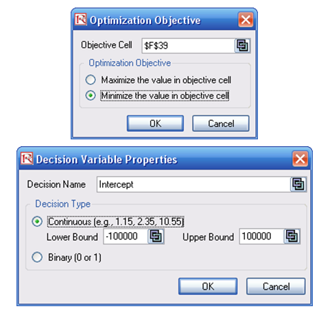
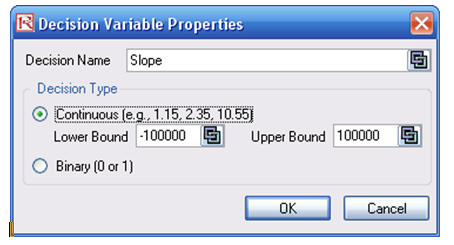
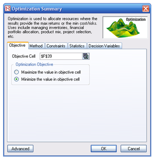
Figure 103.2: Setting up the least squares optimization
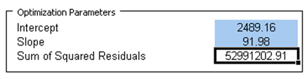
Figure 103.3: Optimized OLS results
The intercept is 2489.16 and the slope is 91.98, which means that the predicted regression equation is Y = 2489.16 + 91.89X. We can also recover these values if we computed these coefficients manually. The region B44 to G66 shows the manual computations and the results are shown in cells C71 and C72, which are identical to those computed using the optimization procedure (Figure 103.4).
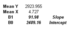
Figure 103.4: Manual computations
The third and perhaps easiest alternative is to use Risk Simulator’s Multiple Regression module. Perform the regression using these steps:
- Select the Y and X values(including the header). That is, select the area B12:C34.
- Click on Risk Simulator | Forecasting | Multiple Regression Analysis.
- Make sure Y is selected as the dependent variable and click OK.
The results are generated as the Report worksheet in this file. Clearly, the regression report is a much more comprehensive than what we have done, complete with analytics and statistical results. The regression results using Risk Simulator shows the same values as we have computed using the two methods shown in Figure 103.5. Spend some time reading through the regression report.
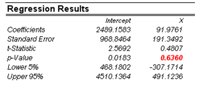
Figure 103.5: Risk Simulator results
Using Risk Simulator is a lot simpler and provides more comprehensive results than the alternative methods. In fact, the t-test shows that X is statistically not significant and hence is a worthless predictor of Y. This is a fact that we cannot determine using the first two methods. Indeed, when you have multiple independent X variables in multivariate regression, you cannot compute the results manually using the second method. The only recourse and best alternative is to use this regression module.