This section on Forecast Prediction (see Figures 7.1, 7.2, and 7.3) includes a sophisticated Business Analytics and Business Statistics module with over 250 functionalities. Start by entering the data in Step 1 (copy and paste from Excel or other ODBC-compliant data source, manually type in data, or click on the Options | Load Example button to load a sample dataset complete with previously saved models). Then, choose the analysis to perform in Step 2 and, using the variables list provided, enter the desired variables to model given the chosen analysis (if you previously clicked Options | Load Example, you can double-click to use and run the saved models in Step 4 to see how variables are entered in Step 2, and use that as an example for your analysis). Click RUN in Step 3 when ready to obtain the Results, Charts, and Statistics of the analysis. You can also Save your model in Step 4 by giving it a name for future retrieval.
The following provides a few quick getting started steps on running the Forecast Prediction module and details on each of the elements in the software, and refer to Dr. Johnathan Mun’s Modeling Risk, Third Edition with dedicated chapters explaining and exploring some of the most critical statistical methodologies available in this module. Feel free to explore the power of this Forecast Prediction module by loading the preset Options | Load Example or watch the Video to quickly get started using the module and review the user manual for more details on the 250 analytical methods. All 250 models are in ROV BizStats, while selected forecasting models are in this current PEAT software.
Forecast Prediction
- Proceed to the Forecast Prediction tab and click on Options | Load Example to load a sample data and model profile or type in your data or copy/paste from another software such as Excel or Word/text file into the data grid in Step 1 (Figure 7.1). You can add your own notes or variable names in the first Notes FBrow.
- Select the relevant model to run in Step 2 and using the example data input settings, enter in the relevant variables. Separate variables for the same parameter using semicolons and use a new line (hit Enter to create a new line) for different parameters.
- Click Run to compute the results. You can view any relevant analytical results, charts, or statistics from the various tabs in Step 3.
- If required, you can provide a model name to save into the profile in Step 4. Multiple models can be saved in the same profile. Existing models can be edited or deleted and rearranged in order of appearance, and all the changes can be saved.
- If you use your own data and create your own models, you can save these models in Step 4.
- If you are playing with the example data/models and need to recover your saved data and models, click on Options | Recover My Models.
- Saving your data and multiple models in Step 4 will result in their being saved as part of the *rovprojecon In addition, if you click on Options| Save/Open Profile, you can save the data and models as a stand-alone *.bizstats file that can be opened in a separate software, ROV BizStats.
TIPS on Using Forecast Prediction
- The data grid size can be set in the Grid Configure button, where the grid can accommodate up to 1,000 variable columns with 1 million rows of data per variable. The pop-up menu also allows you to change the language and decimal settings for your data.
- To get started, it is always a good idea to load the example file that comes complete with some data and precreated models. You can double-click on any of these models to run them and the results are shown in the report area, which sometimes can be a chart or model statistics. Using this example file, you can now see how the input parameters are entered based on the model description, and you can proceed to create your own custom models.
- Click on the variable headers to select one or multiple variables at once, and then right-click to add, delete, copy, paste, or visualize the variables selected.
- Models can also be entered using a Command console (Figure 7.3). To see how this works, double-click to run a model and go to the Command console. You can replicate the model or create your own and click Run Command when ready. Each line in the console represents a model and its relevant parameters.
- Click on the data grid’s column header(s) to select the entire column(s) or variable(s), and once selected, you can right-click on the header to Auto Fit the column, or to Cut, Copy, Delete, or Paste data. You can also click on and select multiple column headers to select multiple variables and right-click and select Visualize to chart the data.
- If a cell has a large value that is not completely displayed, click on and hover your mouse over that cell and you will see a pop-up comment showing the entire value, or simply resize the variable column (drag the column to make it wider, double-click on the column’s edge to auto fit the column, or right-click on the column header and select Auto Fit).
- Use the up, down, left, and right keys to move around the grid, or use the Home and End keys on the keyboard to move to the far left and far right of a row. You can also use combination keys such as Ctrl+Home to jump to the top left cell, Ctrl+End to the bottom right cell, Shift+Up/Down to select a specific area, and so forth.
- You can enter short notes for each variable in the Notes row.
- Try out the various chart icons on the Visualize tab to change the look and feel of the charts(e.g., rotate, shift, zoom, change colors, add legend, etc.).
- The Copy button is used to copy the Results, Charts, and Statistics tabs in Step 3 after a model is run. If no models are run, then the Copy function will only copy a blank page.
- The Report button will only run if there are saved models in Step 4 or if there are data in the grid, otherwise the report generated will be empty. You will also need Microsoft Excel to be installed to run the data extraction and results reports, and Microsoft PowerPoint available to run the chart reports.
- When in doubt about how to run a specific model or statistical method, start the Options| Load Example profile and review how the data is set up in Step 1 or how the input parameters are entered in Step 2. You can use these as getting started guides and templates for your own data and models.
- Click the Options| Load Example button to load a sample set of previously saved data and models. Then double-click on one of the Saved Models in Step 4. You can see the saved model that is selected, and the input variables used in Step 2. The results will be computed and shown in the Step 3 results area, and you can view the Results, Charts, or Statistics depending on what is available based on the model you chose and ran.
- The Grid Configure button allows you to change the number of rows or columns of the data grid in Step 1.
- Click Report only if you need it. That is, this function will run all of the saved models in Step 4 and extract the results to Microsoft Excel, Word, and PowerPoint. We say do it only if you mean it because if you have too many saved models, it will run all models and the entire process might take a few minutes to complete.
- You can save a model if required after setting up the model (entering the data, selecting the model, and configuring the input parameters in Step 2) after you give it a Name in Step 4 and click Save. You can Edit or Delete saved models later.
- You can copy data from another software, such as Microsoft Excel, and paste it into the data grid in Step 1. Simply copy the data, click on the location you wish the data to be pasted into, right-click, and select Paste.
- If your data contains large values (e.g., 10,000,000.00), right-click anywhere in the data grid and select Auto Fit All Columns.
- You can select a variable in the data grid by clicking on the header(s). For instance, you can click on VAR1 and it will select the entire variable.
- When a variable is selected, click on the Visualize button or right-click and select Visualize, and the data will be collapsed into a time-series chart.
- Depending on the model run, sometimes the results will return a chart (e.g., a stochastic process forecast was created, and the results are presented both in the Results subtab and the Charts subtab).
- The charts subtab has multiple chart icons you can use to change the appearance of the chart (e.g., modify the chart type, chart line colors, chart view, etc.).
- Sometimes you can also quickly run multiple models using direct commands (e.g., using the Command Console.
- For new users, we recommend setting up the models using the user interface, starting from Step 1 through to Step 4.
- To start using the console, create the models you need, then click on the Command subtab, copy/edit/replicate the command syntax (e.g., you can replicate a model multiple times and change some of its input parameters very quickly using the command approach), and when ready, click on the Run Command button.
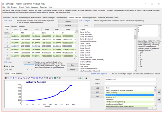
Figure 7.1 – Forecast Prediction: Module Overview
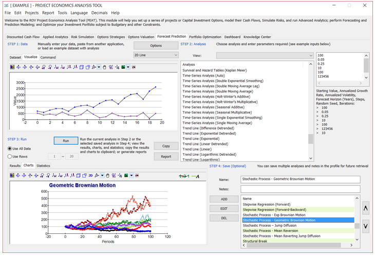
Figure 7.2 – Forecast Prediction: Data Visualization and Results Charts
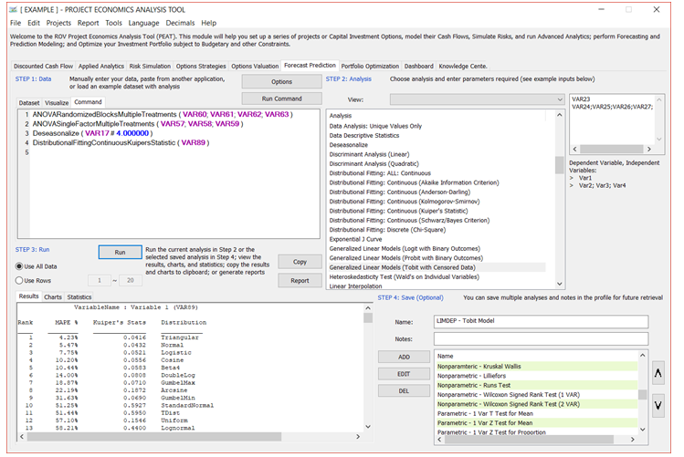
Figure 7.3 – Forecast Prediction: Command Console