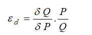
This section illustrates another sample model from the ROV Modeling Toolkit. This model is used to find the optimal pricing levels that will maximize revenues through the use of historical elasticity levels. The price elasticity of demand is a basic concept in microeconomics, which can be briefly described as the percentage change of quantity divided by the percentage change in prices. For example, if, in response to a 10% fall in the price of a good, the quantity demanded increases by 20%, the price elasticity of demand would be 20% / (−10 %) = −2. In general, a fall in the price of a good is expected to increase the quantity demanded, so the price elasticity of demand is negative but in some literature, the negative sign is omitted for simplicity (denoting only the absolute value of the elasticity). We can use this concept in several ways, including the point elasticity by taking the first derivative of the inverse of the demand function and multiplying it by the ratio of price to quantity at a particular point on the demand curve:
where ε is the price elasticity of demand, P is price, and Q is the quantity demanded. Instead of using instantaneous point elasticities, this example uses the discrete version, where we define elasticity as:
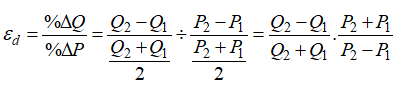
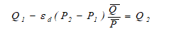
To further simplify things, we assume that in a category of hotel rooms, cruise ship tickets, airline tickets, or any other products with various categories (e.g., standard room, executive room, suite, etc.), there is an average price and average quantity of units sold per period. Therefore, we can further simplify the equation to:
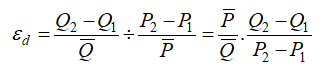
where we now use the average price and average quantity demanded values ![]() If we have in each category the average price and average quantity sold, as in the model, we can compute the expected quantity sold given a new price provided we have the historical elasticity of demand values. See Figure 17.15.
If we have in each category the average price and average quantity sold, as in the model, we can compute the expected quantity sold given a new price provided we have the historical elasticity of demand values. See Figure 17.15.
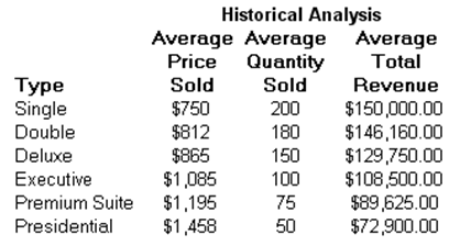
Figure 17.15: Sample Historical Pricing
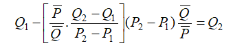
In other words, if we take:
we would get:
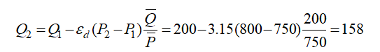
To illustrate, suppose the price elasticity of demand for a single room during high season at a specific hotel property is 3.15 (we use the absolute value), where the average price last season was $750, and the average quantity of rooms sold was 200 units. What would happen if prices were to change from $750 (P1) to $800 (P2)? That is, what would happen to the quantity sold from 200 units (Q1)? See Figure 17.16. Note that ε is a negative value but we simplify it as a positive value here to be consistent with economic literature.
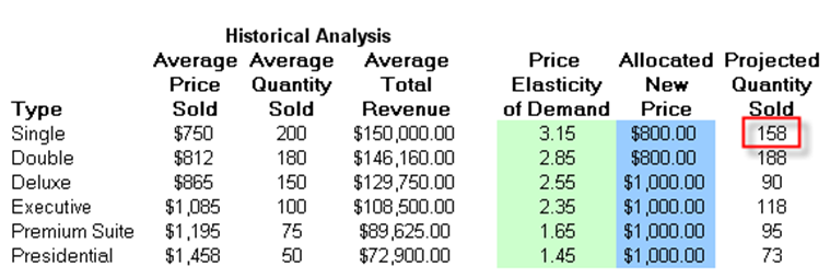
Figure 17.16: Elasticity Simulation
Using the preceding equation, we compute the newly predicted quantity demanded at $800 per night to be:
The higher the price, the lower the quantity demanded, and vice versa. Indeed, the entire demand curve can be reconstructed by applying different price levels. For instance, the demand curve for the single room is reconstructed in Figure 17.17.
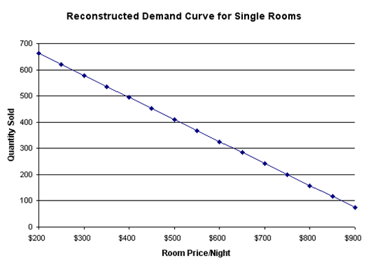
Figure 17.17: Reconstructed Demand Curve for Single Rooms
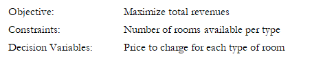
Optimization Procedures
Using the principles of price elasticity of demand, we can now figure out the optimal pricing structure of these hotel rooms by setting:
This model already has the optimization set up. To run it directly, do the following:
- Go to the Model worksheet and click on Risk Simulator | Change Profile and choose the Optimal Pricing with Elasticity profile.
- Click on the Run Optimization icon or click on Risk Simulator | Optimization | Run Optimization.
- Select the Method tab and select either Static Optimization if you wish to view the resulting optimal prices or Stochastic Optimization to run the simulation with optimization multiple times, to obtain a range of optimal prices.
The results from a stochastic optimization routine are seen in the Report worksheet. In addition, several forecast charts will be visible once the stochastic optimization routine completes. For instance, looking at the Executive suites, select Two-Tail, type 90 in the Certainty box, and hit TAB on the keyboard to obtain the 90% confidence level (e.g., the optimal price to charge for the season is between $991 and $993 per night). See Figure 17.18.
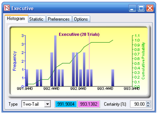
Figure 17.18: Distribution of Stochastic Optimization Decision Variable
To reset the model manually, do the following:
- Go to the Model worksheet, click on Risk Simulator | New Profile, and give the new profile a name.
- Reset the values on prices. That is, enter 800 for cells H7, H8 and 1000 for cells H9 to H12. We choose these values so that we determine the initial starting prices that are easy to remember, versus the optimized price levels later on.
- Set the objective. Select cell J15 and click on the O (set objective) icon or click Risk Simulator | Optimization | Set Objective.
- Set the decision variables. Select cell H7 and click on the D (set decision variable) icon or click Risk Simulator | Optimization | Set Decision. Select Continuous and give it the relevant lower and upper bounds (see columns M and N) or click on the link icons and link the lower and upper bounds (cells M7 and N7).
- Set the constraints. Click on the C icon or Risk Simulator | Optimization | Constraints and add the capacity constraints on the maximum number of available rooms (e.g., click ADD and link cell I7 and make it “<= 250 ” and so forth.
- Click on the Run Optimization icon or click on Risk Simulator | Optimization | Run Optimization.
- Select the Method tab and select either Static Optimization if you wish to view the resulting optimal prices, or Stochastic Optimization to run simulation with optimization multiple times, to obtain a range of optimal prices. But remember that to run a stochastic optimization procedure, you need to have assumptions set up. Select cell G7 and click on Risk Simulator | Set Input Assumption and set an assumption of your choice or choose Normal distribution and use the default values. Repeat for cells G8 to G12, one at a time, and then you can run a stochastic optimization.