Figure 17A.1 illustrates a quick example using Microsoft’s historical stock prices for computing the annualized return and annualized volatility risk. It shows the stock prices for Microsoft downloaded from Yahoo! Finance, a publicly available free resource (you can start by visiting http://finance.yahoo.com and then entering a stock symbol, e.g., MSFT for Microsoft, then click on Quotes: Historical Prices, select Weekly, and select the period of interest to download the data to a spreadsheet for analysis). The data in columns A and B are downloaded from Yahoo. The formula in cell D3 is simply LN(B3/B4) to compute the natural logarithmic value of the relative returns week after week, and is copied down the entire column. The formula in cell E3 is STDEV(D3:D54)*SQRT(52), which computes the annualized (by multiplying the square root of the number of weeks in a year) volatility (by taking the standard deviation of the entire 52 weeks of the year 2004 data). The formula in cell E3 is then copied down the entire column to compute a moving window of annualized volatilities. The volatility used in this example is the average of a 52-week moving window, which covers 2 years of data; that is, cell M8’s formula is AVERAGE(E3:E54), where cell E54 has the following formula: STDEV(D54:D105)*SQRT(52), and, of course, row 105 is January 2003. This means that the 52-week moving window captures the average volatility over a 2-year period and it will smooth the volatility such that infrequent but extreme spikes will not dominate the volatility computation. Of course, a median volatility should also be computed. If the median is far off from the average, the distribution of volatilities is skewed, and the median should be used, otherwise, the average should be used. Finally, these 52 volatilities can be fed into Monte Carlo simulation, using the Risk Simulator software’s custom distribution to run a nonparametric simulation or to perform data fitting procedure to find the best-fitting distribution to simulate.
In contrast, we can compute the annualized returns either using the arithmetic average method or the geometric average method. Cell G3 computes the absolute percentage return for the week where the formula for the cell is (B3–B4)/B4, and the formula is copied down the entire column. Then, the moving average window is computed in cell H3 as AVERAGE(G3:G54)*52, where the average weekly returns are obtained and annualized by multiplying it with 52, the number of weeks in a year. Note that averages are additive and can be multiplied directly by the number of weeks in a year versus volatility, which is not additive. Only volatility squared is additive, which means that the periodic volatility computed previously needs to be multiplied by the square root of 52. The arithmetic average return in cell M14 is, hence, the average of a 52-week period of the moving average computed as AVERAGE(H3:H54). Similarly, the geometric average return is the average of the 52-week moving window of the geometric returns, that is, cell M15 is simply AVERAGE(I3:I54), where in cell I3, we have (POWER(B3/B54,1/52)-1)*52, the geometric average computation. The arithmetic growth rate is typically higher than the geometric growth rate when the returns from period to period are volatile. Typically, the geometric growth rate (with a moving average window) should be used.
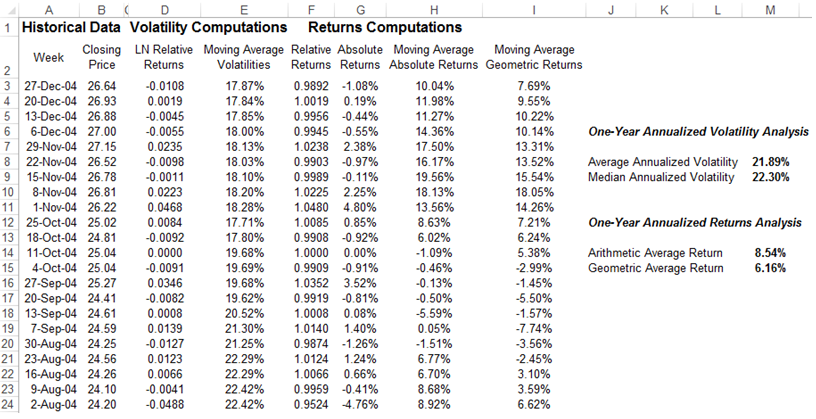
Figure 17A.1: Computing Annualized Return and Risk