File Name: Decision Analysis – Economic Order Quantity and Optimal Manufacturing
Location: Modeling Toolkit | Decision Analysis | Economic Order Quantity and Optimal Manufacturing
Brief Description: Computes the Economic Order Quantity (EOQ) for inventory purposes and simulates an EOQ model to obtain confidence intervals for optimal quantities to order
Requirements: Modeling Toolkit, Risk Simulator
Modeling Toolkit Functions Used: MTZEOQ, MTZEOQOrders, MTZEOQProbability, MTZEOB, MTZEOBBatch, MTZEOBProductionCost, MTZEOBHoldingCost, MTZEOBTotalCost
Economic Order Quantity (EOQ) models define the optimal quantity to order that minimizes total variable costs required to order and hold in inventory or the optimal quantities to manufacture. EOQ models provide several key insights. The most important one is that the optimal order quantity Q* varies with the square root of annual demand, and not directly with annual demand. This fact provides an important economy of scale. For instance, if demand doubles, the optimal inventory does not double but goes up by the square root of 2, or approximately 1.4. This also means that inventory rules based on time-supply are not optimal. For example, a simple rule like inventory managers having to maintain a “month’s worth” of inventory can lead to dangerously low inventory or inventory shortage situations. If demand doubles, then a month’s worth of inventory is twice as large. As noted, this is more quantity than is optimal; a doubling in demand should optimally increase inventory only by the square root of 2, or about 1.4 times.
The EOQ model is a lot more than simple inventory computations, as it computes the optimal quantity to order and the number of orders per year on average, as well as the probability that a product will be out of stock, providing a risk assessment of the probability some items will be out (Figure 26.1). The inputs can be subjected to Monte Carlo simulation using Risk Simulator. For instance, any of the inputs such as demand level or cost of placing an order can be set as input assumptions and the EOQ as the output forecast.
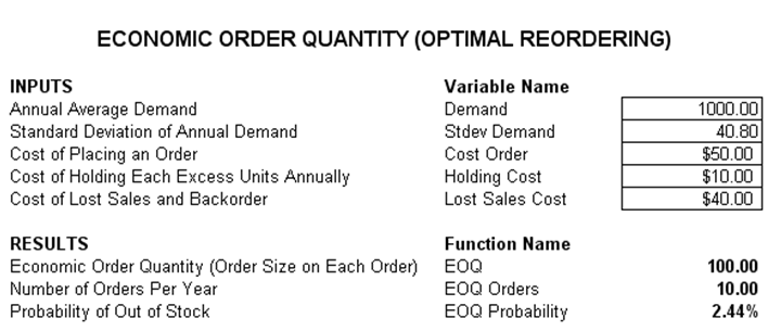
Figure 26.1: EOQ and optimal reordering
The EOQ model also can be extended to cover manufacturing outputs, specifically, finding the optimal quantities to manufacture given assumed average demand levels, production capacity, cost of setting up production, holding cost of inventory, and so forth (Figure 26.2). These two models are fairly self-explanatory and use preprogrammed functions in the Modeling Toolkit software.
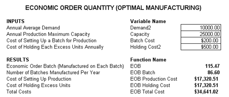
Figure 26.2: EOQ and optimal manufacturing
Procedure
This model already has Monte Carlo simulation predefined using Risk Simulator. To run this model, simply click on Risk Simulator | Change Simulation Profile and select the EOQ Model profile, then click on Risk Simulator | Run Simulation. However, if you wish you can create your own simulation model:
- Start a new simulationprofile and add various assumptions on Demand, Cost of Placing an Order, Holding Cost, and Cost of Lost Sales.
- Add forecaststo the key outputs, such as EOQ or EOQ Probability.
- Run the simulationand interpret the resulting forecast charts as usual.