File Name: Analytics – Central Limit Theorem
Location: Modeling Toolkit | Analytics | Central Limit Theorem
Brief Description: Illustrates the concept of the Central Limit Theorem and the Law of Large Numbers using Risk Simulator’s set assumptions functionality, where many distributions, at the limit, are shown to approach normality
Requirements: Modeling Toolkit, Risk Simulator
This example shows how the Central Limit Theorem works by using Risk Simulator and without the applications of any mathematical derivations. Specifically, we look at how the normal distribution sometimes can be used to approximate other distributions and how some distributions can be made to be highly flexible, as in the case of the beta distribution.
The Central Limit Theorem contains a set of weak-convergence results in probability theory. Intuitively, they all express the fact that any sum of many independent and identically distributed random variables will tend to be distributed according to a particular attractor distribution. The most important and famous result is called the Central Limit Theorem, which states that if the sum of the variables has a finite variance, then it will be approximately normally distributed. As many real processes yield distributions with finite variance, this theorem explains the ubiquity of the normal distribution. Also, the distribution of an average tends to be normal, even when the distribution from which the average is computed is decidedly not normal.
Discrete Uniform Distribution
In this model, we look at various distributions and see that over a large sample size and various parameters, they approach normality. We start off with a highly unlikely candidate, the discrete uniform distribution, also known as the equally likely outcomes distribution, where the distribution has a set of N elements, and each element has the same probability (Figure 1.1). This distribution is related to the uniform distribution, but its elements are discrete instead of continuous. The input requirement is such that minimum < maximum and both values must be integers. An example would be tossing a single die with 6 sides. The probability of hitting 1, 2, 3, 4, 5, or 6 is exactly the same: 1/6. So, how can a distribution like this be converted into a normal distribution?
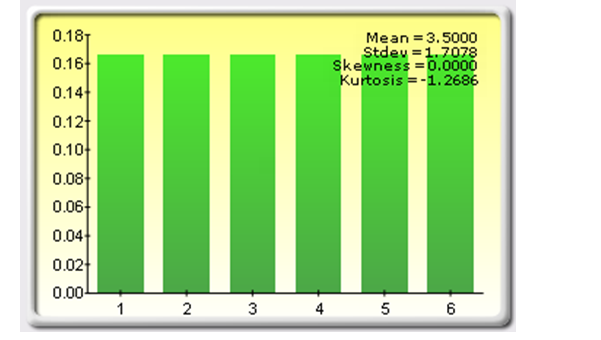
Figure 1.1: Tossing a single die and the discrete uniform distribution
The idea lies in the combination of multiple distributions. Suppose you now take a pair of dice and toss them. You would have 36 possible outcomes, that is, the first single die can be 1 and the second die can be 1, or perhaps 1-2, or 1-3, and so forth, until 6-6, with 36 outcomes as shown in Figure 1.2. 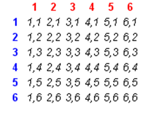
Figure 1.2: Tossing two dice
Now, summing up the two dice, you get an interesting set of results (Figure 1.3).
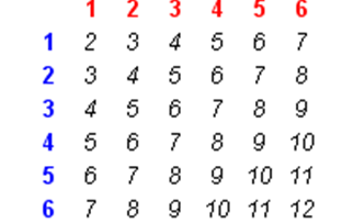
Figure 1.3: Summation of two dice
If you then plotted out these sums, you get an approximation of a normal distribution (Figure 1.4).
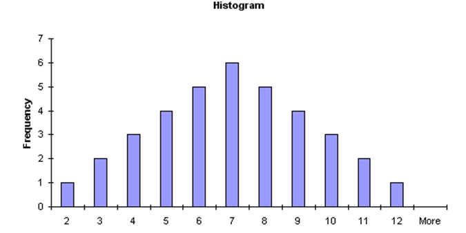
Figure 1.4: Approximation to a normal distribution
In fact, if you threw 12 dice together and added up their values, and repeated the process many times, you get an extremely close discrete normal distribution. If you add 12 continuous uniform distributions, where the results can, say, take on any continuous value between 1 and 6, you obtain a perfectly normal distribution.
Poisson, Binomial, and Hypergeometric Distributions
Continuing with the examples, we show that for higher values of the distributional parameters (where many trials exist), these three distributions also tend to normality. For instance, in the Other Discrete worksheet in the model, notice that as the number of trials (N) in a binomial distribution increases, the distribution tends to normal. Even with a small probability (P) value, as the number of trials N increases, normality again reigns (Figure 1.5). In fact, as N × P exceeds about 30, you can use the normal distribution to approximate the binomial distribution. Also, this is important, as at high N values, it is very difficult to compute the exact binomial distribution value, and the normal distribution is a lot easier to use.
We can test this approximation by using the Distribution Analysis tool (Risk Simulator | Distribution Analysis). As an example, we test a binomial distribution with N = 5000 and P = 0.50. We then compute the mean of the distribution, NP = 2500, and the standard deviation of the binomial distribution,
![]()
We then enter these values in the normal distribution and look at the Cumulative Distribution Function (CDF) of some random range. Sure enough, the probabilities we obtain are close although not precisely the same (Figure 1.6).
The normal distribution does in fact approximate the binomial distribution when N × P is large (compare the results in Figures 1.6 and 1.7).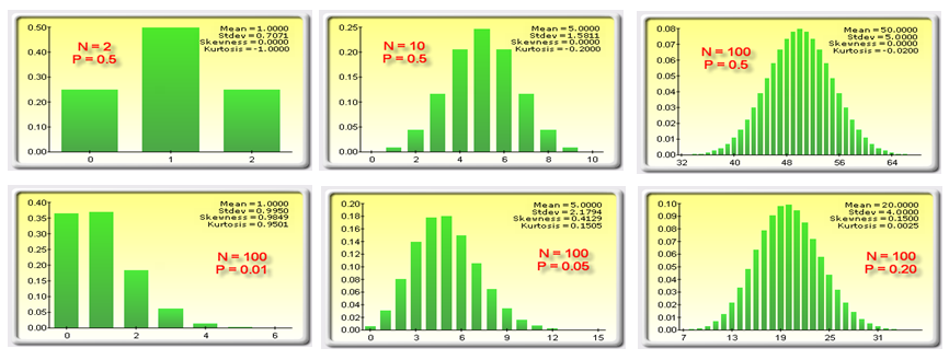
Figure 1.5: Different faces of a binomial distribution
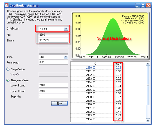
Figure 1.6: Normal approximation of the binomial
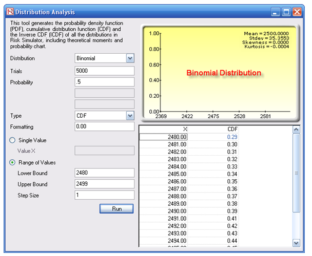
Figure 1.7: Binomial approximation of the normal
The examples also examine the hypergeometric and Poisson distributions. A similar phenomenon occurs: When the input parameters are large, they revert to the normal approximation. In fact, the normal distribution also can be used to approximate the Poisson and hypergeometric distributions. Clearly, there will be slight differences in value as the normal is a continuous distribution whereas the binomial, Poisson, and hypergeometric are discrete distributions. Therefore, slight variations will obviously exist.
Beta Distribution
Finally, the Beta worksheet illustrates an interesting distribution, the beta distribution. Beta is a highly flexible and malleable distribution and can be made to approximate multiple distributions. If the two input parameters, alpha and beta, are equal, the distribution is symmetrical. If either parameter is 1 while the other parameter is greater than 1, the distribution is triangular or J-shaped. If alpha is less than beta, the distribution is said to be positively skewed (most of the values are near the minimum value). If alpha is greater than beta, the distribution is negatively skewed (most of the values are near the maximum value).