- Related AI/ML Methods: Dimension Reduction Factor Analysis
- Related Traditional Methods: Principal Component Analysis, Factor Analysis
Principal component analysis, or PCA, makes multivariate data easier to model and summarize. To understand PCA, suppose we start with N variables that are unlikely to be independent of one another, such that changing the value of one variable will change another variable. PCA modeling will replace the original N variables with a new set of M variables that are less than N but are uncorrelated to one another, while at the same time, each of these M variables is a linear combination of the original N variables so that most of the variation can be accounted for using fewer explanatory variables.
PCA is a way of identifying patterns in data and recasting the data in such a way as to highlight their similarities and differences. Patterns of data are very difficult to find in high dimensions when multiple variables exist, and higher dimensional graphs are very difficult to represent and interpret. Once the patterns in the data are found, they can be compressed, and the number of dimensions is now reduced. This reduction of data dimensions does not mean much reduction in loss of information. Instead, similar levels of information can now be obtained by a fewer number of variables.
PCA is a statistical method that is used to reduce data dimensionality using covariance analysis among independent variables by applying an orthogonal transformation to convert a set of correlated variables data into a new set of values of linearly uncorrelated variables named principal components. The number of computed principal components will be less than or equal to the number of original variables. This statistical transformation is set up such that the first principal component has the largest possible variance accounting for as much of the variability in the data as possible, and each subsequent component has the highest variance possible under the constraint that it is orthogonal to or uncorrelated with the preceding components. Thus, PCA reveals the internal structure of the data in a way that best explains the variance in the data. Such a dimensional reduction approach is useful to process high-dimensional datasets while still retaining as much of the variance in the dataset as possible. PCA essentially rotates the set of points around their mean to align with the principal components. Therefore, PCA creates variables that are linear combinations of the original variables. The new variables have the property that the variables are all orthogonal. Factor analysis is similar to PCA, in that factor analysis also involves linear combinations of variables using correlations, whereas PCA uses covariance to determine eigenvectors and eigenvalues relevant to the data using a covariance matrix. Eigenvectors can be thought of as preferential directions of a dataset or main patterns in the data. Eigenvalues can be thought of as quantitative assessments of how much a component represents the data. The higher the eigenvalues of a component, the more representative it is of the data.
As an example, PCA is useful when running multiple regression or basic econometrics when the number of independent variables is large or when there is significant multicollinearity in the independent variables. It can be run on the independent variables to reduce the number of variables and to eliminate any linear correlations among the independent variables. The extracted revised data obtained after running PCA can be used to rerun the linear multiple regression or linear basic econometric analysis. The resulting model will usually have slightly lower R-squared values but potentially higher statistical significance (lower p-value). Users can decide to use as many principal components as required based on the cumulative variance.
Suppose there are k variables, ![]() , there are exactly k principal components,
, there are exactly k principal components, ![]() , and
, and ![]() , where
, where ![]() are the weights or component loadings. The first principal component
are the weights or component loadings. The first principal component ![]() is a linear combination that best explains the total variation, while the second principal component
is a linear combination that best explains the total variation, while the second principal component ![]() is orthogonal or uncorrelated to the first and explains as much as it can of the remaining variation in the data, and so forth, all the way until the final
is orthogonal or uncorrelated to the first and explains as much as it can of the remaining variation in the data, and so forth, all the way until the final ![]() component.
component.
Related to another method called Factor Analysis, PCA makes multivariate data easier to model and summarize. Figure 9.64 illustrates an example where we start with 5 independent variables that are unlikely to be independent of one another, such that changing the value of one variable will change another variable. Recall that this multicollinearity effect can cause biases in a multiple regression model. Both principal component and factor analysis can help identify and eventually replace the original independent variables with a new set of smaller variables that are less than the original but are uncorrelated to one another, while, at the same time, each of these new variables is a linear combination of the original variables. This means most of the variation can be accounted for by using fewer explanatory variables. Similarly, factor analysis is used to analyze interrelationships within large numbers of variables and simplifies said factors into a smaller number of common factors. The method condenses information contained in the original set of variables into a smaller set of implicit factor variables with minimal loss of information. The analysis is related to the principal component analysis by using the correlation matrix and applying principal component analysis coupled with a varimax matrix rotation to simplify the factors.
The data input requirement is simply the list of variables you want to analyze (separated by semicolons for individual variables or separated by a colon for a contiguous set of variables, such as VAR29:VAR33 for all 5 variables).

We started with 5 independent variables, which means the factor analysis or principal component analysis results will return a 5×5 matrix of eigenvectors and 5 eigenvalues. Typically, we are only interested in components with eigenvalues >1. Hence, in the results, we are only interested in the first three or four factors or components (some researchers would plot these eigenvalues and call it a scree plot, which can be useful for identifying where the kinks are in the eigenvalues).
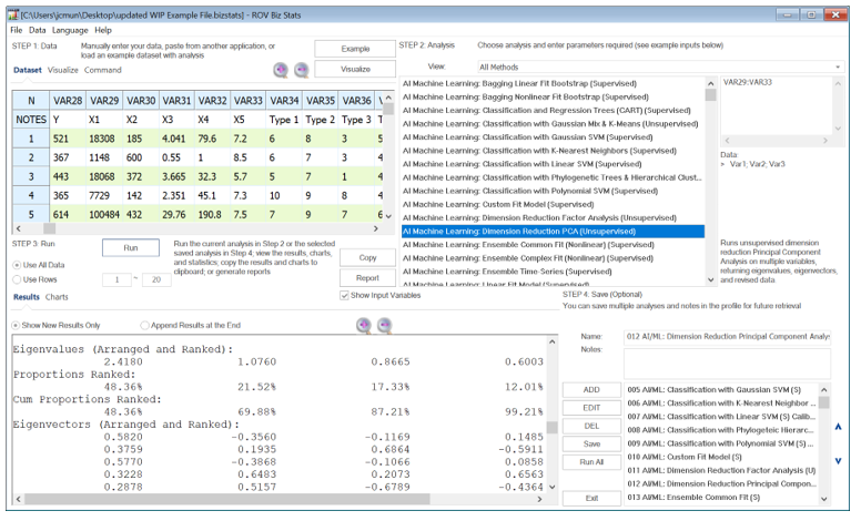
Figure 9.64: AI/ML Dimension Reduction PCA (Unsupervised)
Notice that the first and second factors (the first two result columns) return a cumulative proportion of 69.88%. This means that using these two factors will explain approximately 70% of the variation in all the independent factors themselves. Next, we look at the absolute values of the eigenvalue matrix. It seems that variables 1 and 3 can be combined into a new variable in factor 1, with variables 4 and 5 as the second factor. This can be done separately and outside of principal component analysis. Notice that the results are not as elegant with only 5 variables. The idea of PCA and Factor Analysis is that the more variables you have, the better the algorithm will perform in terms of reducing the number of data variables or the data dimensionality size.
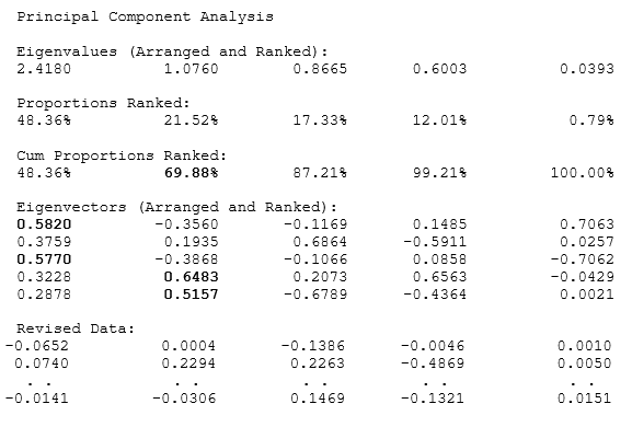
Figure 9.65 shows the results of multiple linear regressions to illustrate how orthogonality works in PCA. For instance, the first multiple regression is run using the original dataset (VAR28 against VAR29:VAR33). The second regression is run based on the revised PCA data (VAR28 against the converted data). Notice that the goodness-of-fit measures such as R-square, Adjusted R-square, Multiple R, and Standard Error of the Estimates are identical. The estimated coefficients will differ because different data were used in each situation. Some of the variables are not significant in the models because this is only meant as an illustration of the PCA method and not about calibrating a good regression model. In fact, using the reduced model, the Adjusted R-square of only using two variables is 23% as opposed to 25% using all 5 independent variables in the original dataset. This showcases the power of PCA, where fewer variables are used while retaining a high level of variability explained.
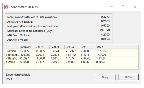
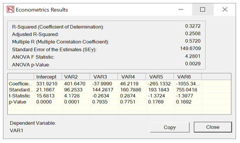
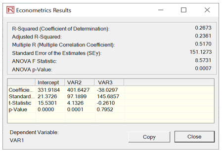
Figure 9.65: PCA Regression Comparability