As shown previously, probability of default is a key parameter for computing credit risk of a portfolio. In fact, the Basel III/IV and III Accords require the probability of default as well as other key parameters such as the loss given default (LGD) and exposure at default (EAD), be reported as well. The reason is that a bank’s expected loss is equivalent to:
Expected Losses = (Probability of Default) × (Loss Given Default) × (Exposure at Default)
or simply: EL = PD × LGD × EAD
PD and LGD are both percentages, whereas EAD is a value. As we have shown how to compute PD in the previous section, we will now revert to some estimations of LGD. There are again several methods used to estimate LGD. The first is through a simple empirical approach where we set LGD = 1 – Recovery Rate. That is, whatever is not recovered at default is the loss at default, computed as the charge off (net of recovery) divided by the outstanding balance: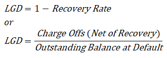
Therefore, if market data or historical information is available, LGD can be segmented by various market conditions, types of obligors, and other pertinent segmentations (use Risk Simulator’s segmentation tool to perform this). LGD can then be readily read off a chart.
A second approach to estimate LGD is more attractive in that if the bank has available information, it can attempt to run some econometric models to create the best-fitting model under an ordinary least squares approach. By using this approach, a single model can be determined and calibrated, and this same model can be applied under various conditions, and no data mining is required. However, in most econometric models, a normal transformation will have to be performed first. Suppose the bank has some historical LGD data (Figure 2.7), then the best-fitting distribution can be found using Risk Simulator by first selecting the historical data, and then clicking on Risk Simulator | Analytical Tools | Distributional Fitting (Single Variable) to perform the fitting routine. The example’s result is a beta distribution for the thousands of LGD values. The p-value can also be evaluated for the goodness-of-fit of the theoretical distribution (i.e., the higher the p-value, the better the distributional fit; so in this example, the historical LGD fits a beta distribution 81% of the time, indicating a good fit).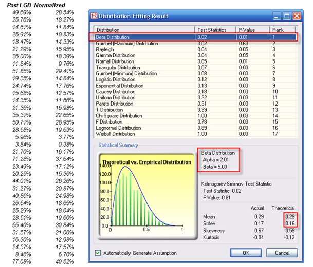
Figure 2.7: Fitting Historical LGD Data
Next, using the Distribution Analysis tool in Risk Simulator, obtain the theoretical mean and standard deviation of the fitted distribution (Figure 2.8). Then, transform the LGD variable using the MTNormalTransform function in the Modeling Toolkit software. For instance, the value of 49.69% will be transformed and normalized to 28.54% (Figure 2.7). Using this newly transformed dataset, you can now run some nonlinear econometric models to determine LGD.
The following is a partial list of independent variables that might be significant for a bank, in terms of determining and forecasting the LGD value:
- Debt to capital ratio
- Profit margin
- Revenue
- Current assets to current liabilities
- Risk rating at default and one year before default
- Industry
- Authorized balance at default
- Collateral value
- Facility type
- Tightness of covenant
- Seniority of debt
- Operating income to sales ratio (and other efficiency ratios)
- Total asset, total net worth, total liabilities
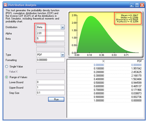
Figure 2.8: Distributional Analysis Tool