File Name: Optimization – Capital Investments (Part B)
Location: Modeling Toolkit | Optimization | Investment Capital Allocation – Part II
Brief Description: Finds the optimal levels of capital investments in a strategic plan based on different risk and return characteristics of each type of product line as applied in an efficient frontier, and the contribution to the entire portfolio’s credit risk is determined
Requirements: Modeling Toolkit, Risk Simulator
This model, Part B of the Capital Investments example, is the second of two parts, continued from the previous chapter. To get started, please first review Part A of the model before attempting to run this follow-up model. This follow-up model looks at a twist at the optimization procedures performed in Part A by now incorporating risk and the return to risk ratio (Sharpe Ratio, a Nobel Prize winning concept). As can be seen in Figure 99.1, the model is the same as Figure 98.1, with the exception of the inclusion of Column F, which is a measure of risk. This risk measure can be a probability of failure or volatility computation. Typically, for a project, the higher the expected value, the higher the risk. Therefore, with the inclusion of this risk value, we can now compute not only the expected returns for the portfolio, but also the expected risk for the entire portfolio, weighted to the various investment levels.
Simply maximizing returns in the portfolio (Opt Run 1 in Figure 99.1, based on the previous chapter’s model) will, by definition, create a potentially higher risk portfolio (high risk equals high return). Instead, we may also want to maximize the Sharpe Ratio (portfolio returns to risk ratio), which will, in turn, provide the maximum levels of return subject to the least risk, or for the same risk, provide the highest returns, yielding an optimal point on the Markowitz Efficient Frontier for this portfolio (Opt Run 2 in Figure 99.1). As can be seen in the optimization results table, Opt Run 1 provides the highest returns ($246,072) as opposed to the original value of $231,058. Nonetheless, Opt Run 2, where we maximize the Sharpe Ratio instead, provides a slightly lower return ($238,816) but the total risk for the entire portfolio is reduced to 4.055% instead of 4.270%. A simulation is run on the original investment allocation, Opt Run 1, and Opt Run 2, and the results are shown in Figure 99.2. Here, we clearly see that the slightly lower returns provide a reduced level of risk, which is good for the bank.
To run this predefined optimization model, simply click on Risk Simulator | Optimization | Run Optimization and click OK. To change the objective from Maximizing Returns to Risk, to Maximizing Returns, simply click on the Objective O icon in the Risk Simulator toolbar or click on Risk Simulator | Optimization | Set Objective and link it to either cell C20 for Sharpe Ratio, or C17, for Returns, and then run the optimization.
In addition, the total investment budget allowed can be changed to analyze what happens to the returns and risk of the portfolio. For instance, Figure 99.3 illustrates the results from such an analysis, and the resulting expected risk and return values. In order to better understand each point’s risk structure, optimization is carried out and a simulation is run. Further down, two sample extreme cases where $2.91M versus $3.61M are invested. From the results, one can see that the higher the risk (higher range of outcomes), the higher the returns (expected values are higher and the probability of beating the original expected value is also higher). Such analyses will provide the bank the ability to better analyze the risk and return characteristics.
Many additional analyses can be applied to this model. For instance, we can apply the Probability of Default computations of implied Asset Value and Implied Volatility to obtain the Cumulative Default Probability so that the bank can understand the risk of this deal and decide (based on the portfolio of deals) what the threshold of lending should be. For instance, if the bank does not want anything above a 3.5% probability of default for a 5-year cumulative loan, then $3.41M is the appropriate loan value threshold. In addition, Value at Risk for a portfolio of loans can also be determined for before and after this new loan, enabling the bank to decide if absorbing this new loan is possible, and the effects on the entire portfolio’s VaR valuation and capital adequacy. Figure 99.4 shows some existing loans (grouped by tranches and types), and the new loan request. It is up to management to decide if the additional hit to capital requirements is reasonable. For details on credit risk analysis and Value at Risk models, please refer to the relevant chapters in this book.
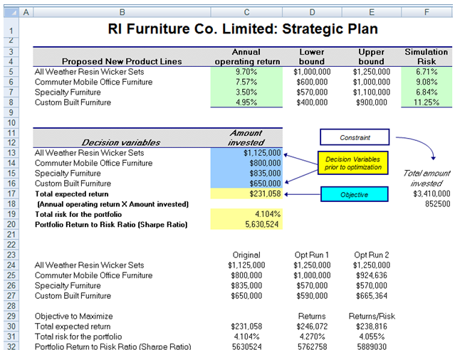
Figure 99.1: Revised capital investment model with the inclusion of stochastic risk elements
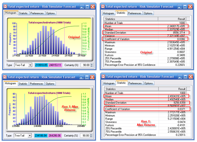
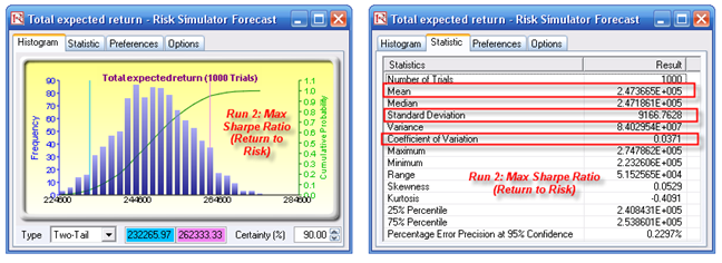
Figure 99.2: Simulation results from optimization runs
Figure 99.3: Efficient frontier results
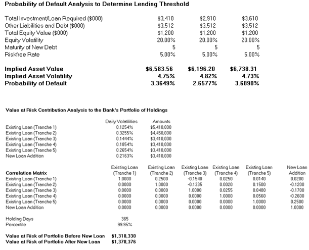
Figure 99.4: Probability of default and contributions to portfolio Value at Risk