When both seasonality and trend exist, more advanced models are required to decompose the data into their base elements: a base case level (L) weighted by the alpha parameter (α); a trend component (b) weighted by the beta parameter (β); and a seasonality component (S) weighted by the gamma parameter (γ). Several methods exist but the two most common are the Holt–Winters additive seasonality and Holt–Winters multiplicative seasonality methods.
Holt–Winters Additive Seasonality
Figures 12.18 and 12.19 illustrate the required computations for determining a Holt–Winters additive forecast model. The Holt–Winters additive seasonality model is a combination of the seasonal additive and double exponential-smoothing models described previously. Similar to seasonal additive and seasonal multiplicative models, the difference between the two Holt–Winters models is that the additive model uses addition and subtraction versus multiplication and division, and, of course, the optimized α, β, and γ parameters would also be different to compensate for these differences in mathematical operations. Figure 12.18 shows the setup of the algorithm, starting from the historical time-serijes data or Actual column, followed by the Level, Trend, and Seasonality columns. The Holt–Winters algorithm assumes that any time-series data can be decomposed into these three components, each with its own weighting schema, set between 0 and 1 inclusive, namely, α for the strength of the Level, β for the strength of the Trend, and γ for the strength of the Seasonality effects. In other words, each of the weights can take on any value between 0% and 100%. The calculations proceed as usual and can be seen in more detail in Figure 12.19.
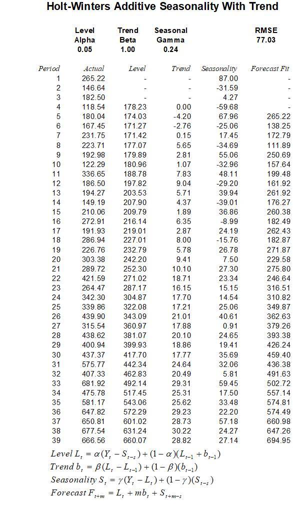
Figure 12.18: Holt–Winters Additive
Figures 12.18 and 12.19 show the Holt–Winters additive model. The first-period value of Level (L) is computed as the average of 265.22, 146.64, 182.50, and 118.54 or 178.23. All subsequent Levels are calculated as![]() or 0.0493 × (180.04 – 87) + (1 – 0.0493) × (178.23 + 0) = 174.03 (as an example for period 5). The optimized α = 0.0493, β = 1.0000, and γ= 0.2351.
or 0.0493 × (180.04 – 87) + (1 – 0.0493) × (178.23 + 0) = 174.03 (as an example for period 5). The optimized α = 0.0493, β = 1.0000, and γ= 0.2351.
The Trend (b) calculation starts at period ![]() or in this case, starting in period 5, we use the equation
or in this case, starting in period 5, we use the equation![]() All subsequent calculations proceed the same way. For instance, the Trend for period 6 is such that we have 1.00 × (171.27 – 174.03) + (1 – 1.00) × (–4.2) = –2.76, and so forth.The Seasonality (S) factor for all periods within
All subsequent calculations proceed the same way. For instance, the Trend for period 6 is such that we have 1.00 × (171.27 – 174.03) + (1 – 1.00) × (–4.2) = –2.76, and so forth.The Seasonality (S) factor for all periods within ![]() (in this case,
(in this case, ![]() is 4), the Seasonality is computed as
is 4), the Seasonality is computed as ![]() or Actual(t)–Level(s) computed to be 265.22 – 178.23 = 87.00 (rounded) for period 1, 146.64 – 178.23 = –31.59 for period 2, and so forth. Starting from period
or Actual(t)–Level(s) computed to be 265.22 – 178.23 = 87.00 (rounded) for period 1, 146.64 – 178.23 = –31.59 for period 2, and so forth. Starting from period ![]() , the Seasonality factor becomes
, the Seasonality factor becomes ![]() or computed as 0.2351 × (180.04 – 174.03) + (1 – 0.2351) × 87.00 = 67.96. All subsequent periods use the same calculation approach.Finally, for the Forecast Fit column, compute
or computed as 0.2351 × (180.04 – 174.03) + (1 – 0.2351) × 87.00 = 67.96. All subsequent periods use the same calculation approach.Finally, for the Forecast Fit column, compute ![]() for future forecast period m or 178.23 + (1 × 0) + 87 = 265.22 (rounded) starting from the
for future forecast period m or 178.23 + (1 × 0) + 87 = 265.22 (rounded) starting from the ![]() period. All subsequent periods proceed the same way. Note that m = 1 always when in-sample forecast fit is calculated and use m ≥ 1 when calculating out-of-sample forecasts.
period. All subsequent periods proceed the same way. Note that m = 1 always when in-sample forecast fit is calculated and use m ≥ 1 when calculating out-of-sample forecasts.
Just like the seasonal models discussed previously, this means that the confidence in future forecasts beyond the seasonality periodicity will be less accurate in general, due to insufficient seasonal data, and we, therefore, assume that the seasonality will repeat itself going forward. This is clearly one of the shortcomings of this methodology.
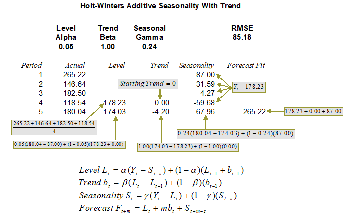
Figure 12.19: Calculating Holt–Winters Additive (Seasonality = 4)
Holt–Winters Multiplicative Seasonality
Figures 12.20 and 12.21 show the required computation for determining a Holt–Winters multiplicative forecast model when both trend and seasonality exist.
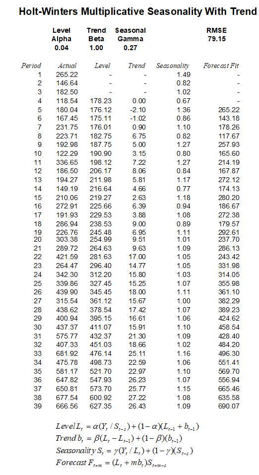
Figure 12.20: Holt–Winters Multiplicative
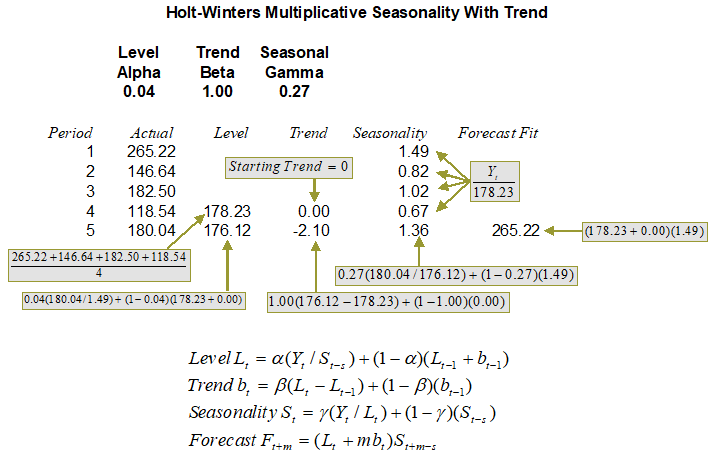
Figure 12.21: Calculating Holt–Winters Multiplicative (Seasonality = 4)