File Names: Six Sigma – Hypothesis Testing and Bootstrap Simulation; Six Sigma – Probabilities and Hypothesis Tests (CDF, PDF, ICDF)
Location: Modeling Toolkit | Six Sigma | Hypothesis Testing and Bootstrap Simulation, and Probabilities and Hypothesis Tests (CDF, PDF, ICDF)
Brief Description: Illustrates how to use Risk Simulator’s Distributional Analysis tool and Modeling Toolkit’s probability functions to obtain exact probabilities of events, and confidence intervals and hypothesis testing for quality control, as well as using Risk Simulator for running hypothesis tests after a simulation run, generating a hypothesis test with raw data, understanding the concept of random seeds, and running a nonparametric bootstrap simulation to obtain the confidence intervals of the statistics
Requirements: Modeling Toolkit, Risk Simulator
Computing Theoretical Probabilities of Events for Sig Sigma Quality Control
In this chapter, we use Risk Simulator’s Distribution Analysis tool and Modeling Toolkit’s functions to obtain exact probabilities of the occurrence of events for quality control purposes. These will be illustrated through some simple discrete distributions. The chapter also provides some continuous distributions for the purposes of theoretical hypotheses tests. Then hypothesis testing on empirically simulated data is presented, where we use theoretical distributions to simulate empirical data and run hypotheses tests. The next chapter goes into more detail on using the Modeling Toolkit’s modules on one-sample and two-sample hypothesis tests using t-tests and Z-tests for values and proportions, analysis of variance (ANOVA) techniques, and some powerful nonparametric tests for small sample sizes. This chapter is a precursor and provides the prerequisite knowledge to the materials presented in the next chapter.
Binomial Distribution
The binomial distribution describes the number of times a particular event occurs in a fixed number of trials, such as the number of heads in 10 flips of a coin or the number of defective items out of 50 items chosen. For each trial, only two outcomes are possible that are mutually exclusive. The trials are independent, where what happens in the first trial does not affect the next trial. The probability of an event occurring remains the same from trial to trial. The probability of success (p) and the number of total trials (n) are the distributional parameters. The number of successful trials is denoted x (the x-axis of the probability distribution graph). The input requirements in the distribution include Probability of success > 0 and < 1 (for example, p ≥ 0.0001 and p ≤ 0.9999) and Number of Trials ≥ 1 and integers and ≤ 1000.
Example: If the probability of obtaining a part that is defective is 50%, what is the probability that in selecting four parts at random, there will be no defective part, or one defective part, or two defective parts, and so forth? Recreate the probability mass function or probability density function (PDF), where we define P(x=0) as the probability (P) of the number of successes of an event (x), and the mathematical combination (C ):
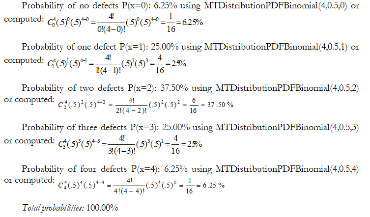
In addition, you can sum up the probabilities to obtain the cumulative distribution function (CDF):
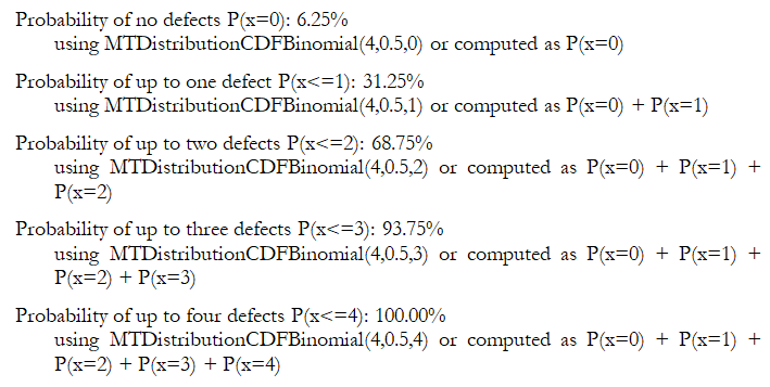
The same analysis can be performed using the Distribution Analysis tool in Risk Simulator. For instance, you can start the tool by clicking on Risk Simulator | Analytical Tools | Distributional Analysis, selecting Binomial, entering in 4 for Trials, 0.5 for Probability, and then selecting PDF as the type of analysis, and a range of between 0 and 4 with a step of 1. The resulting table and PDF distribution are exactly as computed using the Modeling Toolkit functions as seen in Figure 146.1.
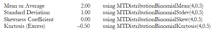
The four distributional moments can also be determined using the tool as well as using the MT functions:
In addition, typically, for discrete distributions, the exact probabilities are called probability mass functions (PMFs); they are called probability density functions (PDFs) for continuous distributions. However, in this book, we use both terms interchangeably. Also, this chapter highlights only some of the examples illustrated in the model. To view more detailed examples, please see the Excel model in the Modeling Toolkit.
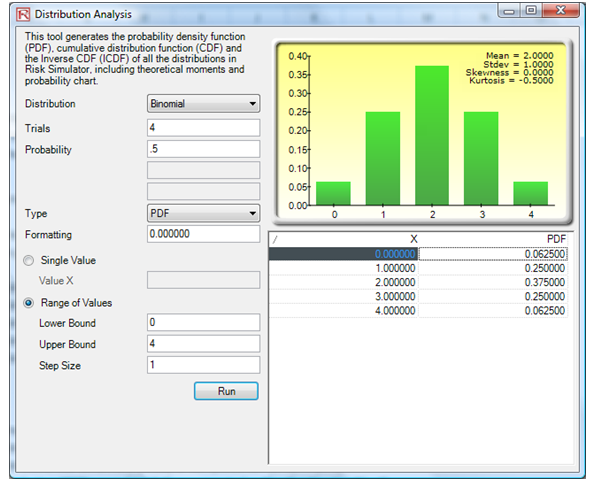
Figure 146.1: Distributional analysis for a binomial PDF
Poisson Distribution
The Poisson distribution describes the number of times an event occurs in a given space or time interval, such as the number of telephone calls per minute or the number of errors per page in a document. The number of possible occurrences in any interval is unlimited; the occurrences are independent. The number of occurrences in one interval does not affect the number of occurrences in other intervals, and the average number of occurrences must remain the same from interval to interval. Rate or Lambda is the only distributional parameter. The input requirements for the distribution are Rate > 0 and ≤ 1000.
Example: A tire service center has the capacity of servicing six customers in an hour. From prior experience, on average three show up an hour. The owner is afraid that there might insufficient manpower to handle an overcrowding of more than six customers. What is the probability that there will be exactly six customers? What about six or more customers?
Using the Distribution Analysis tool, we see that the PDF of exactly six customers is 5.04% (Figure 146.2) and the probability of six or more is the same as 1 – the CDF probability of five or less, which is 1 – 91.61% or 8.39% (Figure 146.3).
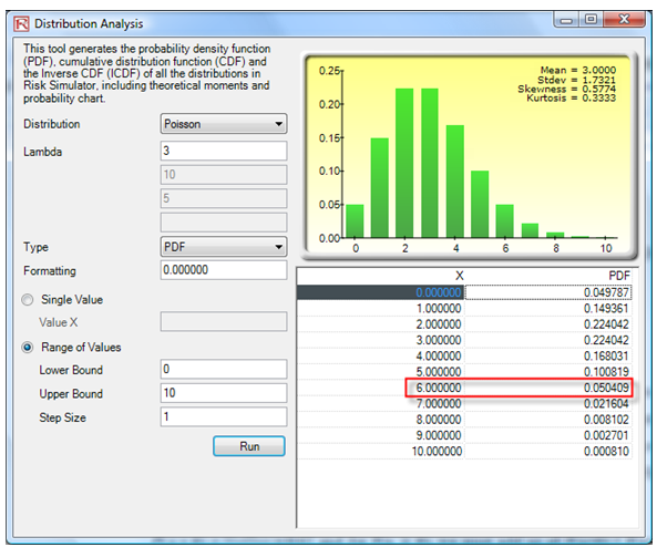
Figure 146.2: PDF on a Poisson
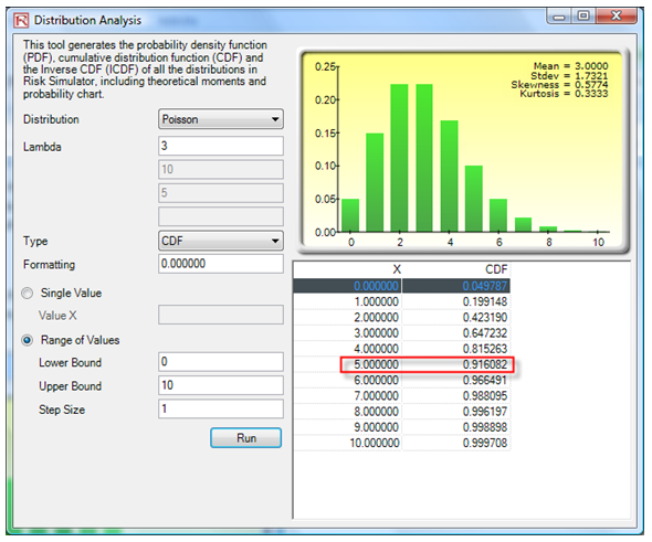
Figure 146.3: CDF on a Poisson
C. Normal Distribution
The normal distribution is the most important distribution in probability theory because it describes many natural phenomena, such as people’s IQs or heights. Decision makers can use the normal distribution to describe uncertain variables such as the inflation rate or the future price of gasoline. Some value of the uncertain variable is the most likely (the mean of the distribution), the uncertain variable could as likely be above the mean as it could be below the mean (symmetrical about the mean), and the uncertain variable is more likely to be in the vicinity of the mean than farther away. Mean (μ) and standard deviation (σ) are the distributional parameters. The input requirements are that Mean can take on any value and Standard Deviation > 0 and can be any positive value.
Example: You observe that in the past, on average, your manufactured batteries last for 15 months with a standard deviation of 1.5 months. Assume that the battery life is normally distributed. If a battery is randomly selected, find the probability that it has a life of less than 16.5 months or over 16.5 months.
Using the tool, we obtain CDF of X = 16.5 months as 84.13%, which means that there is an 84.13% chance that the manufactured batteries last up to 16.5 months and 1 – 0.8413 or 15.87% chance the batteries will last over 16.5 months (Figure 146.4). The same value of 84.13% can be obtained using the function MTDistributionCDFNormal(15,1.5,16.5) to obtain 84.13% (Figure 146.5).
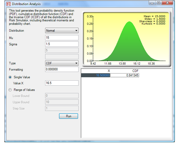
Figure 146.4: CDF of a normal distribution
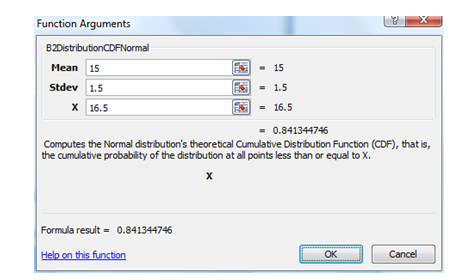
Figure 146.5: CDF of normal using function calls
Example: Alternatively, if you wish to provide a 12-month warranty on your batteries, that is, if the battery dies before 12 months, you will give a full refund. What are the chances that you may have to provide this refund?
Using the tool, we find that the CDF for X = 12 is a 2.28% chance that a refund will have to be issued (Figure 146.6).
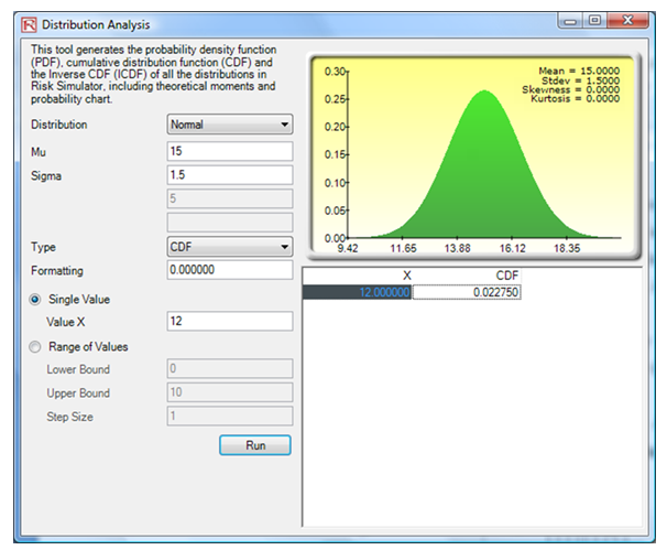
Figure 146.6: Probability of a guaranteed refund
So far, we have been computing the probabilities of events occurring using the PDF and CDF functions and tools. We can also reverse the analysis and obtain the X values given some probability, using the inverse cumulative distribution function (ICDF), as seen next.
Example: If the probability calculated in the preceding example is too high, hence, too costly for you and you wish to minimize the cost and probability of having to refund your customers down to a 1% probability, what would be a suitable warranty date (in months)?
The answer is that to provide anything less than an 11.51-month guarantee will most likely result in less than or equal to a 1% chance of a return. To obtain the results here, we use the ICDF analysis in the Distribution Analysis tool (Figure 146.7). Alternatively, we can use the Modeling Toolkit function MTDistributionICDFNormal(15,1.5,0.01) to obtain 11.510478 (Figure 146.8).
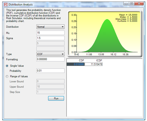
Figure 146.7: Obtaining the inverse cumulative distribution function (ICDF)
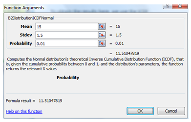
Figure 146.8: Function call for ICDF
Hypothesis Tests in a Theoretical Situation
This section illustrates how to continue using the Distribution Analysis tool to simplify theoretical hypothesis tests.
Example: Sometimes we need to obtain certain X values given a certainty and probability level for the purposes of hypothesis testing. This is where the ICDF comes in handy. For instance, suppose a lightbulb manufacturer needs to test if its bulbs can last on average 1,000 burning hours. If the plant manager randomly samples 100 lightbulbs and finds that the sample average is 980 hours with a standard deviation of 80 hours, at a 5% significance level (two-tails), do the lightbulbs last an average of 1,000 hours?
There are several methods to solve this problem, including the use of confidence intervals, Z-scores, and p-values. For example, we are testing the null hypothesis Ho: Population Mean = 1,000 and the alternate hypothesis Ha: Population Mean is NOT 1,000. Using the Z-score approach, we first obtain the Z-score equivalent to a two-tail alpha of 5% (which means one tail is 2.5%, and using the Distribution Analysis tool we get the Z = 1.96 at a CDF of 97.50%, equivalent to a one-tail p-value of 2.5%). Using the Distribution Analysis tool, set the distribution to Normal with a mean of zero and standard deviation of 1 (this is the standard normal Z distribution). Then, compute the ICDF for 0.975 or 97.5% CDF, which provides an X value of 1.9599 or 1.96 (Figure 146.9).
Using the confidence interval formula, we get:
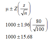
This means that the statistical confidence interval is between 984.32 and 1015.68. As the sample mean of 980 falls outside this confidence interval, we reject the null hypothesis and conclude that the true population mean is different from 1,000 hours.
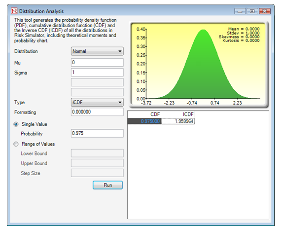
Figure 146.9: Standard normal Z-score
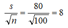
A much quicker and simpler approach is to use the Distribution Analysis tool directly. Seeing that we are performing a statistical sample, we first need to correct for small sampling size bias by correcting the standard deviation to get:
Then, we can find the CDF relating to the sample mean of 980. We see that the CDF p-value is 0.0062, less than the alpha of 0.025 one tail (or 0.50 two tail), which means we reject the null hypothesis and conclude that the population mean is statistically significantly different from the 1,000 hours tested (Figure 146.10).
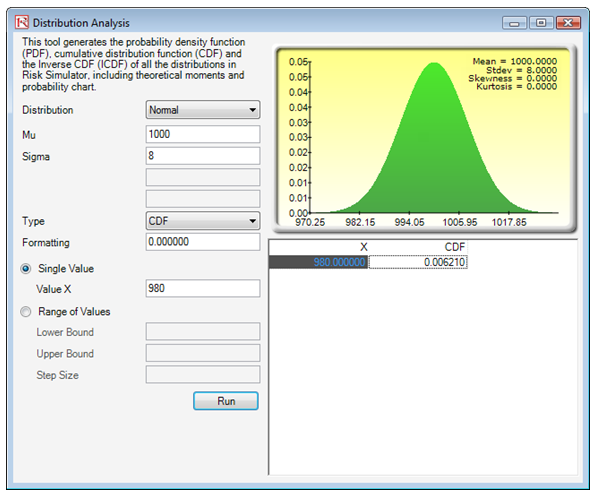
Figure 146.10: Obtaining p-values using the Distribution Analysis tool
Yet another alternative is to use the ICDF method for the mean and sampling adjusted standard deviation and compute the X values corresponding to the 2.5% and 97.5% levels. The results indicate that the 95% two-tail confidence interval is between 984.32 and 1,015.68 as computed previously. Hence, 980 falls outside this range; this means that the sample value of 980 is statistically far away from the hypothesized population of 1,000 (i.e., the unknown true population based on a statistical sampling test can be determined to be not equal to 1,000). See Figure 146.11.

Figure 146.11: Computing statistical confidence intervals
Note that we adjust the sampling standard deviation only because the population is large and we sample a small size. However, if the population standard deviation is known, we do not divide it by the square root of N (sample size).
Example: In another example, suppose it takes on average 20 minutes with a standard deviation of 12 minutes to complete a certain manufacturing task. Based on a sample of 36 workers, what is the probability that you will find someone completing the task taking between 18 and 24 minutes?
Again, we adjust the sampling standard deviation to be 12 divided by the square root of 36 or equivalent to 2. The CDFs for 18 and 24 are 15.86% and 97.72%, respectively, yielding the difference of 81.86%, which is the probability of finding someone taking between 18 and 24 minutes to complete the task. See Figure 146.12.

Figure 146.12: Sampling confidence interval
Example: Sometimes, when the sample size is small, we need to revert to using the Student’s T distribution. For instance, suppose a plant manager studies the life of a particular battery and samples 10 units. The sample mean is 5 hours with a sample standard deviation of 1 hour. What is the 95% confidence interval for the battery life?
Using the T distribution, we set the degrees of freedom as n – 1 or 9, with a mean location of 0 for a standard T distribution. The ICDF for 0.975 or 97.5% (5% two-tail means 2.5% on one tail, creating a complement of 97.5%) is equivalent to 2.262 (Figure 146.13). So, the 95% statistical confidence interval is:
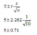
Therefore, the confidence interval is between 4.29 and 5.71.
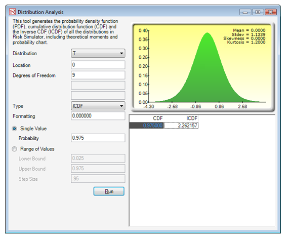
Figure 146.13: Standard T distribution
Hypothesis Tests in an Empirical Simulation
This next example shows how two different forecasts or sets of data can be tested against one another to determine if they have the same means and variances. That is, if the first distribution has a mean of 100, how far away does the mean of the second distribution have to be such that they are considered statistically different? The example illustrates two models (A and B) with the same calculations (see Simulation Model worksheet) where the income is revenue minus cost. Both sets of models have the same inputs and the same distributional assumptions on the inputs, and the simulation is run on the random seed of 123456.
Two major items are noteworthy. The first is that the means and variances (as well as standard deviations) are slightly different. These differences raise the question as to whether the means and variances of these two distributions are identical. A hypothesis test can be applied to answer this first question. A nonparametric bootstrap simulation can also be applied to test the other statistics to see if they are statistically valid. The second item of interest is that the results from A and B are different although the input assumptions are identical and an overall random seed has been applied (Figure 146.14). The different results occur because with a random seed applied, each distribution is allowed to vary independently as long as it is not correlated to another variable. This is a key and useful fact in Monte Carlo simulation.
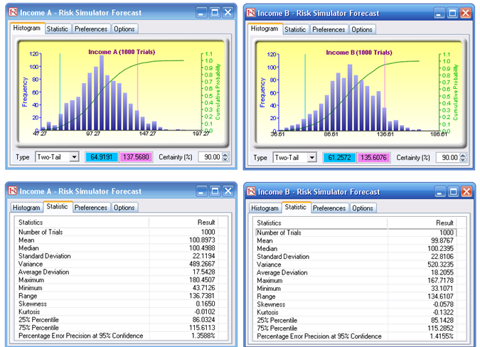
Figure 146.14: Simulation results
Running a Hypothesis Test
To run this model, simply:
- Open the existing simulation profile by selecting Risk Simulator | Change Simulation Profile. Choose the Hypothesis Testing profile.
- Select Risk Simulator | Run Simulation or click on the RUN icon.
- After the simulation run is complete, select Risk Simulator | Analytical Tools | Hypothesis Test.
- Make sure both forecasts are selected and click OK.
The report and results are provided in Figure 146.15. The results indicate that the p-value for the t-test is higher than 0.05, indicating that both means are statistically identical and that any variations are due to random white noise. Further, the p-value is also high for the F-test, indicating that both variances are also statistically identical to one another.
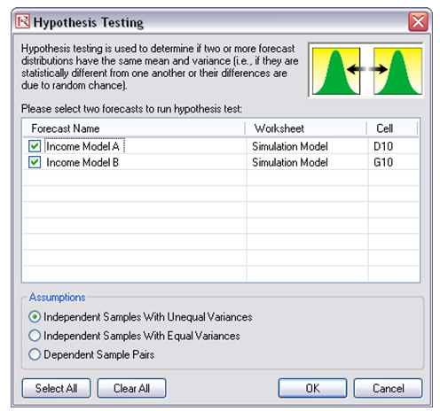
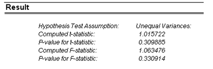
Figure 146.15: Hypothesis testing results
Running a Nonparametric Bootstrap Simulation
The preceding hypothesis test is a theoretical test and is thus more accurate than empirical tests (e.g., bootstrap simulation). However, these tests do not exist for other statistics; hence, an empirical approach is required, namely, nonparametric bootstrap simulation. To run the bootstrap simulation, simply reset and rerun the simulation; then, once the simulation is complete, click on Risk Simulator | Analytical Tools | Nonparametric Bootstrap. Choose one of the forecasts (only one forecast can be chosen at a time when running bootstrap simulation), select the statistics of interest, and click OK (Figure 146.16).
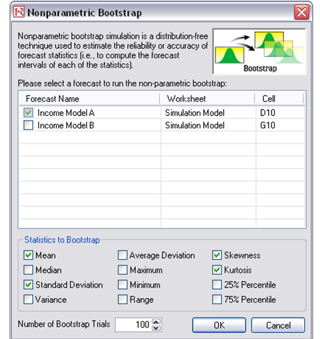
Figure 146.16: Nonparametric bootstrap simulation
The resulting forecast charts are empirical distributions of the statistics. By typing in 90 on the certainty box and hitting TAB on the keyboard, the 90% confidence is displayed for each statistic. For instance, the skewness interval is between 0.0452 and 0.2877, indicating that the value zero is outside this interval; that is, at the 90% two-tail confidence (or significance of 0.10 two-tailed), model A has a statistically significant positive skew. Clearly, the higher the number of bootstrap trials, the more accurate the results (recommended trials are between 1,000 and 10,000). Think of bootstrap simulation in this way: Imagine you have 100 people with the same exact model running the simulation without any seed values. At the end of the simulations, each person will have a set of means, standard deviations, skewness, and kurtosis. Clearly, some people will have exactly the same results while others are going to be slightly off, by virtue of random simulation. The question is, how close or variable is the mean or any of these statistics? In order to answer that question, you collect all 100 means and show the distribution and figure out the 90% confidence level (Figure 146.17). This is what bootstrap does. It creates alternate realities of hundreds or thousands of runs of the same model, to see how accurate and what the spread of the statistic is. This also allows us to perform hypothesis tests to see if the statistic of interest is statistically significant or not.
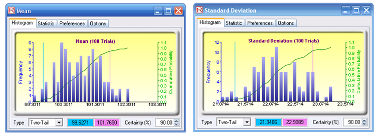
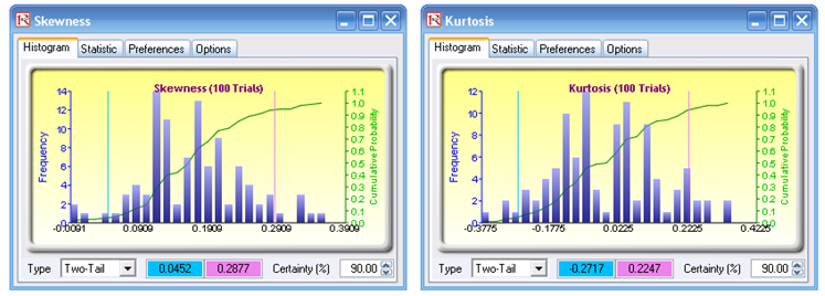
Figure 146.17: Bootstrap simulation’s forecast results