This technical note explains the basics of Convolution Theory and Copula Theory as they apply to probability distributions and stochastic modeling, both in theory and practice. It attempts to show that, in theory, convolution and copulas are elegant and critical in solving basic distributional moments but when it comes to practical applications, these theories are unwieldy and mathematically intractable. Consequently, it is necessary to run empirical Monte Carlo simulations, where the results of said empirical simulations approach the theoretically predicted results at the limit, allowing practitioners a powerful practical toolkit for modeling.
Many probability distributions are both flexible and interchangeable. For example:
- Arcsine and Parabolic distributions are special cases of the Beta distribution.
- Binomial and Poisson distributions approach the Normal distribution at the limit.
- Binomial distribution is a Bernoulli distribution with multiple trials.
- Chi-square distribution is the squared sum of multiple Normal distributions.
- Discrete Uniform distributions’ sum (12 or more) approaches the Normal distribution.
- Erlang distribution is a special case of the Gamma distribution when the alpha shape parameter is positive.
- Exponential distribution is the inverse of the Poisson distribution on a continuous basis.
- F-distribution is the ratio of two chi-square distributions.
- Gamma distribution is related to the Lognormal, Exponential, Pascal, Erlang, Poisson, and chi-square distributions.
- Laplace distribution comprises two Exponential distributions in one.
- Lognormal distribution’s logarithmic values approach the Normal distribution.
- Pascal distribution is a shifted Negative Binomial distribution.
- Pearson V distribution is the inverse of the Gamma distribution.
- Pearson VI distribution is the ratio of two Gamma distribution
- PERT distribution is a modified Beta distribution.
- Rayleigh distribution is a modified Weibull distribution.
- T-distribution with high degrees of freedom (>30) approaches the Normal distribution.
CONVOLUTION
Mathematicians came up with the distributions listed above through the use of convolution, among other methods. As a quick introduction, if there are two independent and identically distributed (i.i.d.) random variables, X and Y, and where their respectively known probability density functions (PDF) are ![]() and
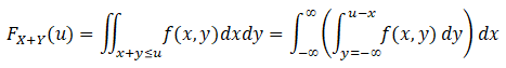
and![]() we can then generate a new probability distribution by combining X and Y using basic summation, multiplication, and division. Some examples are listed above, e.g., the F-distribution is a division of two chi-square distributions, the normal distribution is a sum of multiple uniform distributions, etc. To illustrate how this works, consider the cumulative distribution function (CDF) of a joint probability distribution between the two random variables X and Y:
we can then generate a new probability distribution by combining X and Y using basic summation, multiplication, and division. Some examples are listed above, e.g., the F-distribution is a division of two chi-square distributions, the normal distribution is a sum of multiple uniform distributions, etc. To illustrate how this works, consider the cumulative distribution function (CDF) of a joint probability distribution between the two random variables X and Y:
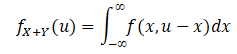
Differentiating the CDF equation above yields the PDF:
Example 1: The convolution of the simple sum of two identical and independent uniform distributions approaches the triangular distribution.
As a simple example, if we take the sum of two i.i.d. uniform distributions with a minimum of 0 and maximum of 1, we have: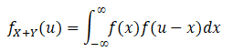
where for a Uniform [0, 1] distribution, , we have:
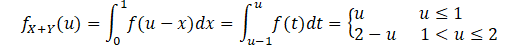
which approaches a simple triangular distribution.
Figure TN.11 shows an empirical approach where two Uniform [0, 1] distributions are simulated for 20,000 trials and their sums added. The computed empirical sums are then extracted and the raw data fitted using the Kolmogorov–Smirnov fitting algorithm in Risk Simulator. The triangular distribution appears as the best-fitting distribution with a 74% goodness-of-fit. As seen in the convolution of only two uniform distributions, the result is a simple triangular distribution.
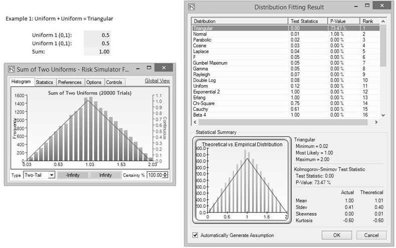
Figure TN.11: Convolution of Two Uniform Distributions via Simulation
Example 2: The convolution simple sum of 12 identical and independent uniform distributions approaches the normal distribution.
If we take the same approach and simulate 12 i.i.d. Uniform [0, 1] distributions and sum them, we would obtain a very close to perfect normal distribution as shown in Figure TN.12, with a goodness-of-fit at 99.3% after running 20,000 simulation trials.
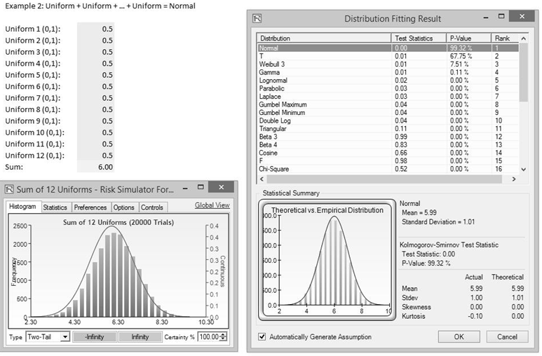
Figure TN.12: Convolution of 12 Uniform Distributions to Create a Normal Distribution
Example 3: The convolution simple sum of multiple identical and independent exponential distributions approaches the gamma (Erlang) distribution.
In this example, we sum two i.i.d. exponential distributions and generalize it to multiple distributions. To get started, we use two identical Exponential [λ = 2] distributions:

where ![]()
is the PDF for the exponential distribution for all x ≥ 0; λ ≥ 0, and the distribution’s mean is β = 1/λ
If we generalize to n random i.i.d. exponential distributions and apply mathematical induction:
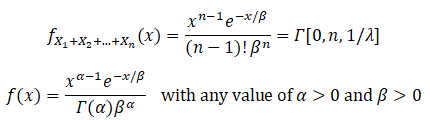
This is, of course, the generalized gamma distribution with α and β for the shape and scale parameters:
![]()
When the β parameter is a positive integer, the gamma distribution is called the Erlang distribution, used to predict waiting times in queuing systems, where the Erlang distribution is the sum of random variables each having a memoryless exponential distribution. Setting n as the number of these random variables, the mathematical construct of the Erlang distribution is:
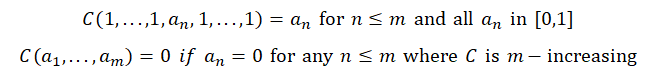
The empirical approach is shown in Figure TN.13, where we have two exponential distributions with λ = 2 (this means that the mean β = 1/λ = 0.5). The sum of these two distributions, after running 20,000 Monte Carlo simulation trials and extracting and fitting the raw simulated sum data (Figure TN.13), shows a 99.4% goodness-of-fit when fitted to the gamma distribution where the α = 2 and β = 0.5 (rounded), corresponding to n = 2 and λ = 2.
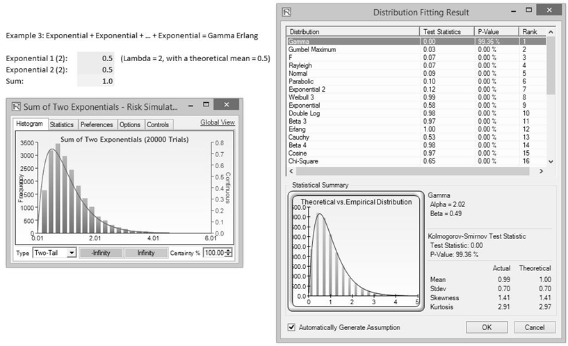
Figure TN.13: Convolution of Exponentials to Create a Gamma Erlang
COPULA
A copula is a multivariate probability distribution for which the marginal probability distribution of each variable is uniform. Copulas are used to describe the dependence between random variables and are typically used to model distributions that are correlated with one another.
The standard definition of copulas is based on Sklar’s Theorem, which states that an m-dimensional copula (or m-copula) is a function C from the unit m-cube [0, 1]m to the unit interval [0, 1] that satisfies the following conditions:
Consider a continuous m-variate distribution function ![]() with univariate marginal distributions
with univariate marginal distributions![]() and inverse quantile functions
and inverse quantile functions ![]() . Then we have where are uniformly distributed variates. Therefore, the transforms of uniform variates are distributed as . This means we have:
. Then we have where are uniformly distributed variates. Therefore, the transforms of uniform variates are distributed as . This means we have:
![]()
where ![]() are uniformly distributed variates. Therefore, the transforms of uniform variates are distributed as
are uniformly distributed variates. Therefore, the transforms of uniform variates are distributed as![]()
This means we have: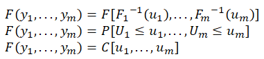
where C is the unique copula associated with the distribution function. That is, y~F , and F is continuous, then
![]()
and if U~C then we have
![]()
Mathematical algorithms using Iman-Conover and Cholesky decomposition matrices are used to compute the joint marginal distributions. Copulas are parametrically specified joint distributions generated from given marginals. Therefore, the properties of copulas are analogous to properties of joint distributions.
PROS AND CONS OF CONVOLUTION AND COPULA
Convolution theory is applicable and elegant for theoretical constructs of probability distributions. With basic addition, multiplication, and division of known i.i.d. distributions, we can determine its theoretical outputs. The issue with convolution theory is that there are no correlations (independently distributed) between the random variables and their distributions, and the individual distributions have to be exactly the same (identically distributed) and commonly known.
Therefore, if one modifies the distributions, uses exotic distributions, mixes and matches different non–i.i.d. distributions, adds correlations, creates large Excel models (beyond the simple addition, multiplication, or division as shown above, such as when there are exotic financial models and computations), and uses truncation, empirical nonparametric distributions, historical simulation, and other combinations of such issues, convolution will not work and cannot predict the outcomes. In addition, both convolution and copula theorems can only be used to compute correlations of joint distributions but would be limited to only a few distributions before the mathematics become intractable due to the large matrix inversions, multiple integrals, and differential equations that need to be solved. Therefore, users are restricted to using Monte Carlo risk simulations.