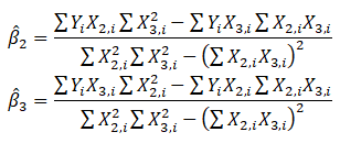
Multicollinearity exists when there is a linear relationship between the independent variables. When this occurs, the regression equation cannot be estimated at all. In near collinearity situations, the estimated regression equation will be biased and provide inaccurate results. This situation is especially true when a step-wise regression approach is used, where the statistically significant independent variables will be thrown out of the regression mix earlier than expected, resulting in a regression equation that is neither efficient nor accurate. As an example, suppose the following multiple regression analysis exists, where ![]()
Then the estimated slopes can be calculated through
Now suppose that there is perfect multicollinearity, that is, there exists a perfect linear relationship between ![]() such that
such that ![]() for all positive values of λ. Substituting this linear relationship into the slope calculations for β2 the result is indeterminate. In other words, we have
for all positive values of λ. Substituting this linear relationship into the slope calculations for β2 the result is indeterminate. In other words, we have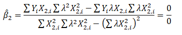
The same calculation and results apply to β3, which means that the multiple regression analysis breaks down and cannot be estimated given a perfect collinearity condition.
One quick test of the presence of multicollinearity in a multiple regression equation is that the R-squared value is relatively high while the t-statistics are relatively low. Another quick test is to create a correlation matrix between the independent variables. A high cross-correlation indicates a potential for multicollinearity. The rule of thumb is that a correlation with an absolute value greater than 0.75 is indicative of severe multicollinearity. Another test for multicollinearity is the use of the variance inflation factor (VIF), obtained by regressing each independent variable to all the other independent variables, obtaining the R-squared value, and calculating the VIF of that variable by estimating:![]()
A high VIF value indicates a high R-squared near unity. As a rule of thumb, a VIF value greater than 10 is usually indicative of destructive multicollinearity.
Another common violation is heteroskedasticity, that is, the variance of the errors increases over time. Figure 9.41 illustrates this case, where the width of the vertical data fluctuations increases or fans out over time. In this example, the data points have been changed to exaggerate the effect. However, in most time-series analyses, checking for heteroskedasticity is a much more difficult task. Figure 9.42 shows a comparative view of homoskedasticity (equal variance of the errors) versus heteroskedasticity.
If the variance of the dependent variable is not constant, then the error’s variance will not be constant. The most common form of such heteroskedasticity in the dependent variable is that the variance of the dependent variable may increase as the mean of the dependent variable increases for data with positive independent and dependent variables.
Unless the heteroskedasticity of the dependent variable is pronounced, its effect will not be severe: the least-squares estimates will still be unbiased, and the estimates of the slope and intercept will either be normally distributed if the errors are normally distributed or at least normally distributed asymptotically (as the number of data points becomes large) if the errors are not normally distributed. The estimate for the variance of the slope and overall variance will be inaccurate, but the inaccuracy is not likely to be substantial if the independent-variable values are symmetric about their mean.
Heteroskedasticity of the dependent variable is usually detected informally by examining the X-Y scatter plot of the data before performing the regression. If both nonlinearity and unequal variances are present, employing a transformation of the dependent variable may have the effect of simultaneously improving the linearity and promoting equality of the variances. Otherwise, a weighted least-squares linear regression may be the preferred method of dealing with a nonconstant variance of the dependent variable.
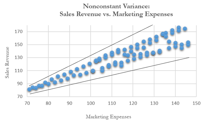
Figure 9.41: Scatter Plot Showing Heteroskedasticity with Nonconstant Variance
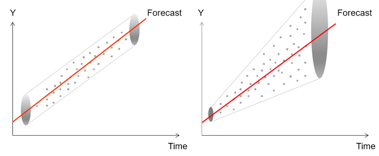
Figure 9.42: Homoskedasticity and Heteroskedasticity
BizStats has several related methods to use when testing for heteroskedasticity. The following lists the main tests. Figure 9.43 illustrates the Breusch–Pagan–Godfrey test. In all the tests, the null hypothesis is always that of homoskedasticity. And, of course, these tests are applicable only to time-series data. These tests can also be used for testing misspecifications and nonlinearities.
The Breusch–Pagan–Godfrey test for heteroskedasticity uses the main model to obtain error estimates and, using squared estimates, a restricted model is run and the Breusch–Pagan–Godfrey test is computed. The Lagrange Multiplier test for heteroskedasticity also uses the main model to obtain error estimates and, using squared estimates, a restricted model is run, and the Lagrange Multiplier test is computed. The Wald–Glejser test for heteroskedasticity again uses the main model to obtain error estimates and, using squared estimates, a restricted model is run and the Wald–Glejser test is computed. The Wald’s Individual Variables test for heteroskedasticity runs multiple tests to see if the volatilities or uncertainties (standard deviation or variance of a variable) are nonconstant over time.
Regardless of the test used, the results typically agree as to whether the null hypothesis can be rejected. If there is disagreement among any of these tests, we typically use the smallest p-value to determine if there is heteroskedasticity.
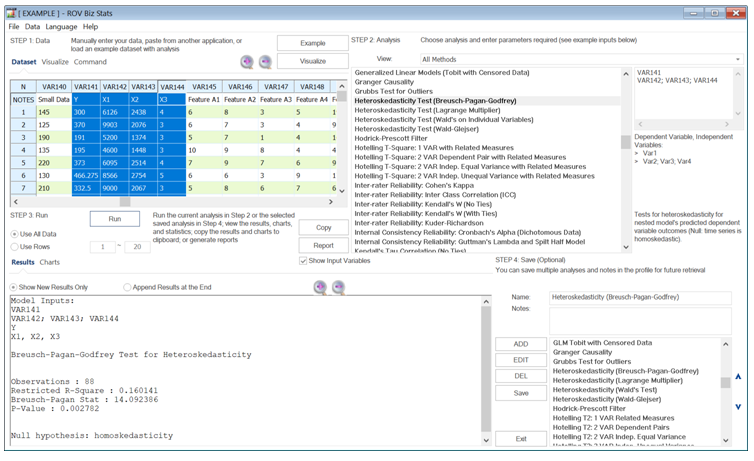
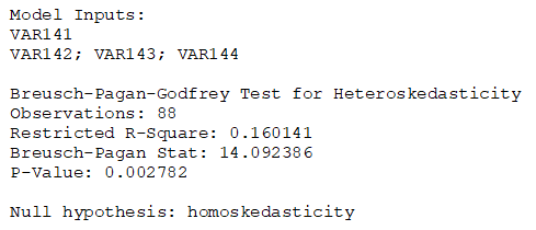
Figure 9.43: Heteroskedasticity Tests