Following are methods of distributional fitting tests:
- Akaike Information Criterion (AIC). Rewards goodness-of-fit but also includes a penalty that is an increasing function of the number of estimated parameters (although AIC penalizes the number of parameters less strongly than other methods).
- Anderson–Darling (AD). When applied to testing if a normal distribution adequately describes a set of data, it is one of the most powerful statistical tools for detecting departures from normality and is powerful for testing normal tails. However, in non-normal distributions, this test lacks power compared to others.
- Kuiper’s Statistic (K). Related to the KS test, making it as sensitive in the tails as at the median and also making it invariant under cyclic transformations of the independent variable, rendering it invaluable when testing for cyclic variations over time. In comparison, the AD test provides equal sensitivity at the tails as the median, but it does not provide the cyclic invariance.
- Schwarz/Bayes Information Criterion (SC/BIC). The SC/BIC test introduces a penalty term for the number of parameters in the model, with a larger penalty than AIC.
The null hypothesis being tested is such that the fitted distribution is the same distribution as the population from which the sample data to be fitted comes. Thus, if the computed p-value is lower than a critical alpha level (typically 0.10 or 0.05), then the distribution is the wrong distribution (reject the null hypothesis). Conversely, the higher the p-value, the better the distribution fits the data (do not reject the null hypothesis, which means the fitted distribution is the correct distribution, or null hypothesis of H0: Error = 0, where the error is defined as the difference between the empirical data and the theoretical distribution). Roughly, you can think of p-value as a percentage explained; that is, for example, if the computed p-value of a fitted normal distribution is 0.9727, then setting a normal distribution with the fitted mean and standard deviation explains about 97.27% of the variation in the data, indicating an especially good fit. Both the results and the report show the test statistic, p-value, theoretical statistics (based on the selected distribution), empirical statistics (based on the raw data), the original data (to maintain a record of the data used), and the assumptions complete with the relevant distributional parameters (i.e., if you selected the option in Risk Simulator to automatically generate assumptions and if a simulation profile already exists). The results also rank all the selected distributions and how well they fit the data.
Figures 9.30 and 9.31 show Risk Simulator’s Distributional Fitting method. The null hypothesis (H0) being tested is such that the fitted distribution is the same distribution as the population from which the sample data to be fitted comes. Thus, if the computed p-value is lower than a critical alpha level (typically 0.10 or 0.05), then the distribution is the wrong distribution. Conversely, the higher the p-value, the better the distribution fits the data. Roughly, you can think of p-value as a percentage explained, that is, if the p-value is 0.9996 (Figure 9.31), then setting a normal distribution with a mean of 100.67 and a standard deviation of 10.40 explains about 99.96% of the variation in the data, indicating an especially good fit. The data was from a 1,000-trial simulation in Risk Simulator based on a normal distribution with a mean of 100 and a standard deviation of 10. Because only 1,000 trials were simulated, the resulting distribution is fairly close to the specified distributional parameters and, in this case, has about a 99.96% precision.
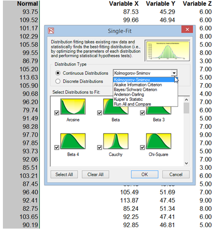
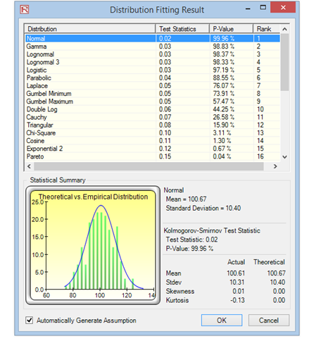
Figure 9.30: Risk Simulator Distribution Fitting Setup
Figure 9.31: Risk Simulator Distribution Fitting Results