- Related AI/ML Methods: Linear Fit Model
- Related Traditional Methods: Basic Econometric Model, Multiple Regression
The AI Machine Learning Custom Fit model is applicable in forecasting time-series and cross-sectional data for modeling relationships among variables. It allows you to create custom-fit multiple regression models. Econometrics refers to a branch of business analytics, modeling, and forecasting techniques for modeling the behavior of or forecasting certain business, financial, economic, physical science, and other variables. Running the Custom Fit model is like regular econometric regression analysis except that the dependent and independent variables can be modified before a regression is run. For more detailed explanations of regression models, see the sections on Linear and Nonlinear Multivariate Regression and Regression Analysis, as well as the associated sections on pitfalls of regression modeling.
As usual, the standard practice is to divide your data into training and testing sets. The training set (one dependent with one or more independent variables) is used to train the algorithm and obtain the best-fitting parameters. In this model, you can create your custom equations (Figure 9.63). Note that only one variable is allowed as the Training Y Dependent Variable, whereas multiple variables are allowed in the Training X Independent Variables section, separated by a semicolon (;), and that basic mathematical functions can be used (e.g., LN, LOG, LAG, +, -, /, *, TIME, RESIDUAL, DIFF). For instance, you can use your training set’s dependent variable as VAR373 and independent variables VAR374; (VAR375)^2; LN(VAR376), and so forth. You need to use the same functional form for the testing set’s independent variables as well (but with the same or different variables), otherwise, the model will not run properly. For example, a complementary set of testing independent variables would be VAR380; (VAR381)^2; LN(VAR382). Notice that the same functional form is used but applied to different variables. Applying it to the same variables would be the same as running a customized econometric model instead.
The algorithm also allows you to optionally enter known testing set dependent values. Sometimes these are known and sometimes they are unknown and are to be forecasted. If the values are unknown, simply leave the input empty or enter a 0 in the input if you wish to enter the next input, which is the forecast results save location in the data grid. Figure 9.63 shows these last two inputs treated as optional and left empty.
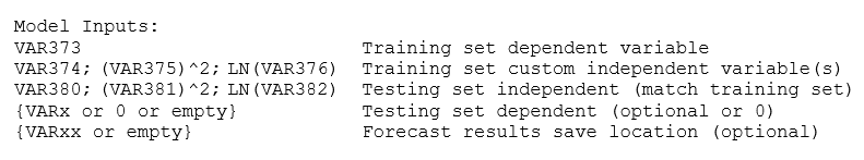
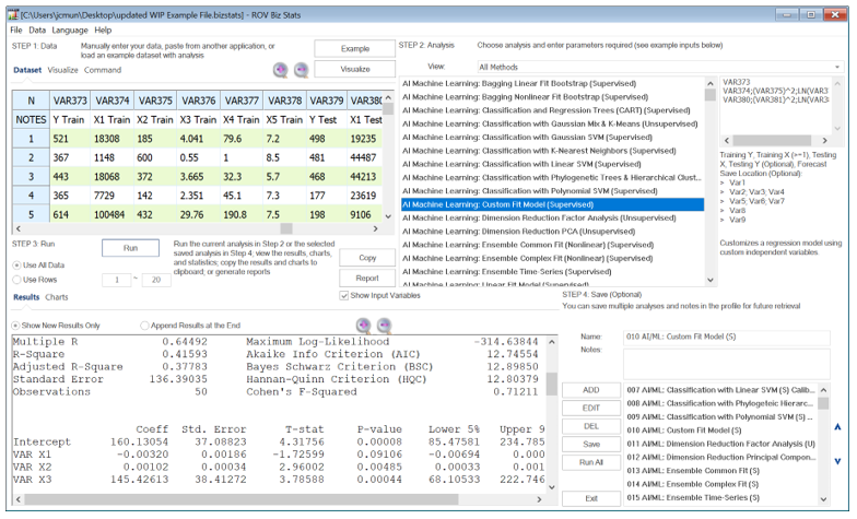
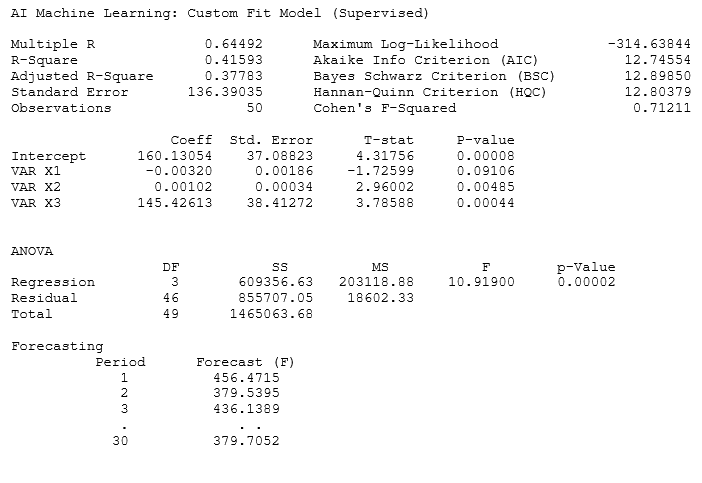
Figure 9.63: AI/ML Custom Fit Model (Supervised)
The results interpretation would be similar to the basic econometric analysis. The goodness-of-fit results and fitted parameter estimations pertain to the training dataset, whereas the forecast values are based on the testing dataset when applied to these fitted parameters. Sometimes, you may wish to hold some data back from the training dataset and apply it to the testing dataset to test the accuracy of the model and its ability to forecast, as well as to view the forecast errors. In other words, the optional testing set’s dependent variable can be used and because these known values are applied, forecast errors can also be generated as a result. For example, the VARx value above can be set to VAR379.