This example illustrates the application of stochastic optimization using a sample model with four asset classes each with different risk and return characteristics. The idea here is to find the best portfolio allocation such that the portfolio’s bang for the buck, or returns to risk ratio, is maximized. That is, the goal is to allocate 100% of an individual’s investment among several different asset classes (e.g., different types of mutual funds or investment styles: growth, value, aggressive growth, income, global, index, contrarian, momentum, etc.). This model is different from others because there exist several simulation assumptions (risk and return values for each asset in columns C and D), as seen in Figure 17.9.
A simulation is run, then optimization is executed, and the entire process is repeated multiple times to obtain distributions of each decision variable. The entire analysis can be automated using Stochastic Optimization.
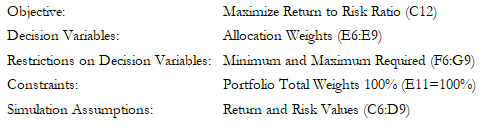
In order to run an optimization, several key specifications on the model have to be identified first:
The model shows the various asset classes. Each asset class has its own set of annualized returns and annualized volatilities. These return and risk measures are annualized values such that they can be consistently compared across different asset classes. Returns are computed using the geometric average of the relative returns, while the risks are computed using the logarithmic relative stock returns approach.
Column E, the Allocation Weights, holds the decision variables, which are the variables that need to be tweaked and tested such that the total weight is constrained at 100% (cell E11). Typically, to start the optimization, we will set these cells to a uniform value. In this case, cells E6 to E9 are set at 25% each. In addition, each decision variable may have specific restrictions in its allowed range. In this example, the lower and upper allocations allowed are 10% and 40%, as seen in columns F and G. This setting means that each asset class may have its own allocation boundaries.
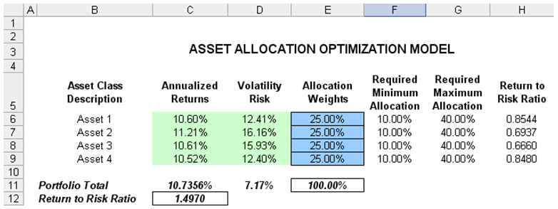
Figure 17.9: Asset Allocation Model Ready for Stochastic Optimization
Next, column H shows the return to risk ratio, which is simply the return percentage divided by the risk percentage for each asset, where the higher this value, the higher the bang for the buck. The remaining parts of the model show the individual asset class rankings by returns, risk, return to risk ratio, and allocation. In other words, these rankings show at a glance which asset class has the lowest risk or the highest return, and so forth.
Running an Optimization
To run this model, simply click on Risk Simulator | Optimization | Run Optimization. Alternatively, and for practice, you can set up the model using the following steps:
- Open the example model at Risk Simulator | Example Models | 13 Stochastic Optimization.
- Start a new profile(Risk Simulator | New Profile).
- For stochastic optimization, set distributional assumptions on the risk and returns for each asset That is, select cell C6, set an assumption (Risk Simulator | Set Input Assumption), and make your own assumption as required. Repeat for cells C7 to D9.
- Select cell E6, define the decision variable (Risk Simulator | Optimization | Set Decision or click on the Set Decision D icon) and make it a Continuous Variable. Then link the decision variable’s name and minimum/maximum required to the relevant cells (B6, F6, G6).
- Then use the Risk Simulator Copy on cell E6, select cells E7 to E9, and use Risk Simulator Paste (Risk Simulator | Copy Parameter and Risk Simulator | Paste Parameter, or use the copy and paste icons). Remember not to use Excel’s regular copy and paste functions.
- Next, set up the optimization’s constraints by selecting Risk Simulator | Optimization | Constraints, selecting ADD, and selecting the cell E11 and making it equal 100% (total allocation, and do not forget the % sign).
- Select cell C12, the objective to be maximized, and make it the objective: Risk Simulator | Optimization | Set Objective or click on the O icon.
- Run the optimization by going to Risk Simulator | Optimization | Run Optimization. Review the different tabs to make sure that all the required inputs in steps 2 and 3 are correct. Select Stochastic Optimization and let it run for 500 trials repeated 20 times (Figure 17.10 illustrates these setup steps).
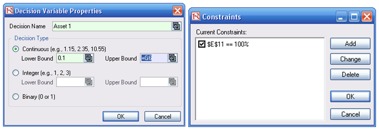
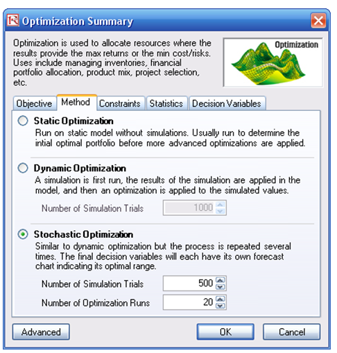
Figure 17.10: Setting Up the Stochastic Optimization Problem
Click OK when the simulation completes and a detailed stochastic optimization report will be generated along with forecast charts of the decision variables.
Viewing and Interpreting Forecast Results
Stochastic optimization is performed when a simulation is first run and then the optimization is run. Then the whole analysis is repeated multiple times. The result is a distribution of each decision variable rather than a single-point estimate (Figure 17.11). So instead of saying you should invest 30.53% in Asset 1, the optimal decision is to invest between 30.19% and 30.88% as long as the total portfolio sums to 100%. This way, the results provide management or decision makers a range of flexibility in the optimal decisions, and all the while accounting for the risks and uncertainties in the inputs.
Notes
- Super Speed Simulation with Optimization. You can also run stochastic optimization with super speed simulation. To do this, first reset the optimization by resetting all four decision variables back to 25%. Next select Run Optimization, click on the Advanced button (Figure 17.10) and select the checkbox for Run Super Speed Simulation. Then, in the run optimization user interface, select Stochastic Optimization on the Method tab and set it to run 500 trials and 20 optimization runs, and click OK. This approach will integrate the super speed simulation with optimization. Notice how much faster the stochastic optimization runs. You can now quickly rerun the optimization with a higher number of simulation trials.
- Simulation Statistics for Stochastic and Dynamic Optimization. Notice that if there are input simulation assumptions in the optimization model (i.e., these input assumptions are required to run the dynamic or stochastic optimization routines), the Statistics tab is now populated in the Run Optimization user interface. You can select from the drop list the statistics you want, such as average, standard deviation, coefficient of variation, conditional mean, conditional variance, a specific percentile, and so forth. Thus, if you run a stochastic optimization, a simulation of thousands of trials will first run; then the selected statistic will be computed, and this value will be temporarily placed in the simulation assumption cell; then an optimization will be run based on this statistic; then the entire process is repeated multiple times. This method is important and useful for banking applications in computing Conditional Value at Risk or Conditional VaR.
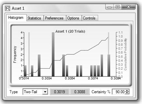
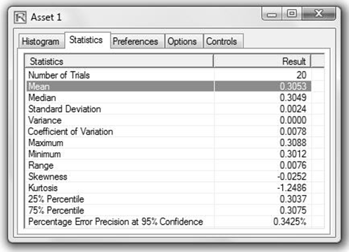
Figure 17.11: Simulated Results from the Stochastic Optimization Approach