File Name: Simulation – Correlation Effects Model
Location: Modeling Toolkit | Risk Simulator | Correlation Effects Model
Brief Description: Illustrates how to use Risk Simulator for creating correlated simulations and comparing the results between correlated and uncorrelated models, as well as extracting and manually computing (verifying) the assumptions’ correlations
Requirements: Modeling Toolkit, Risk Simulator
This model illustrates the effects of correlated simulation compared to uncorrelated simulation, that is, when a pair of simulated assumptions is not correlated, positively correlated, and negatively correlated. Sometimes the results can be very different. In addition, the raw data of the simulated assumptions are extracted after the simulation, and manual computations of their pairwise correlations are performed. The results indicate that the correlations hold after the simulation.
Running a Monte Carlo Simulation
To run this model, simply:
- Click on Correlation model and replicate the assumptionsand forecasts.
- Run the simulationby clicking on the RUN icon or Risk Simulator | Run Simulation.
Viewing and Interpreting Forecast Results
The resulting simulation statistics indicate that the negatively correlated variables provide a tighter or smaller standard deviation or overall risk level on the model. See Figure 135.1.
This relationship exists because negative correlations provide a diversification effect on the variables and hence tend to make the standard deviation slightly smaller. Thus, we need to make sure to input correlations when there indeed are correlations between variables. Otherwise, this interacting effect will not be accounted for in the simulation.
The positive correlation model has a larger standard deviation, as a positive correlation tends to make both variables travel in the same direction, which makes the extreme ends wider and hence increases the overall risk. Therefore, the model without any correlations will have a standard deviation between the positive and negative correlation models.
Notice that the expected value or mean does not change much. In fact, if sufficient simulation trials are run, the theoretical and empirical values of the mean remain the same. The first moment (central tendency) does not change with correlations. Only the second moment (spread) will change.
Note that this characteristic exists only in simple models with a positive relationship. That is, a Price × Quantity model is considered a “positive” relationship model (as is a Price + Quantity model), where a negative correlation decreases the range and a positive correlation increases the range. The opposite is true for negative relationship models. For instance, Price ÷ Quantity or Price – Quantity would be a negative relationship model, and a positive correlation will reduce the range of the forecast variable, whereas a negative correlation will increase the range. Finally, for more complex models (e.g., larger models with multiple variables interacting with positive and negative relationships and sometimes with positive and negative correlations), the results are hard to predict and cannot be determined theoretically. Only by running a simulation would the true results of the range and outcomes be determined. In such a scenario, tornado analysis and sensitivity analysis would be more appropriate.
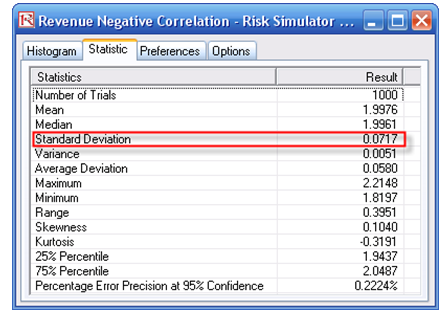
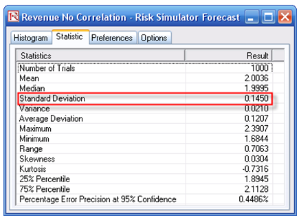
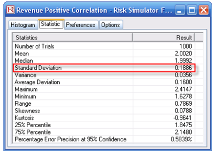
Figure 135.1: Effects on forecast statistics when variables are correlated