In October 2014, the Basel Committee on Banking Supervision released a Basel Consultative Document entitled, “Operational Risk: Revisions to the Simpler Approaches,” and in it describes the concepts of operational risk as the sum product of frequency and severity of risk events within a one-year time frame and defines the Operational Capital at Risk (OPCAR) as the tail-end 99.9% Value at Risk. The Basel Consultative Document describes a Single Loss Approximation (SLA) model defined as![]()
where the inverse of the compound distribution![]() is the summation of the unexpected losses
is the summation of the unexpected losses![]()
and expected losses ![]() λ is the Poisson distribution’s input parameter (average frequency per period; in this case, 12 months); and X represents one of several types of continuous probability distributions representing the severity of the losses (e.g., Pareto, Log Logistic, etc.). The Document further states that this is an approximation model limited to subexponential-type distributions only and is fairly difficult to compute. The X distribution’s cumulative distribution function (CDF) will need to be inverted using Fourier transform methods, and the results are only approximations based on a limited set of inputs and their requisite constraints. Also, as discussed below, the SLA model proposed in the Basel Consultative Document significantly underestimates OPCAR.
λ is the Poisson distribution’s input parameter (average frequency per period; in this case, 12 months); and X represents one of several types of continuous probability distributions representing the severity of the losses (e.g., Pareto, Log Logistic, etc.). The Document further states that this is an approximation model limited to subexponential-type distributions only and is fairly difficult to compute. The X distribution’s cumulative distribution function (CDF) will need to be inverted using Fourier transform methods, and the results are only approximations based on a limited set of inputs and their requisite constraints. Also, as discussed below, the SLA model proposed in the Basel Consultative Document significantly underestimates OPCAR.
This current technical note provides a new and alternative convolution methodology to compute OPCAR that is applicable across a large variety of continuous probability distributions for risk severity and includes a comparison of their results with Monte Carlo risk simulation methods. As will be shown, both the new algorithm using numerical methods to model OPCAR and the Monte Carlo risk simulation approach tends to the same results and seeing that simulation can be readily and easily applied in the CMOL software and Risk Simulator software (source: www.realoptionsvaluation.com), we recommend using simulation methodologies for the sake of simplicity. While the Basel Committee has, throughout its Basel II-III requirements and recommendations, sought after simplicity so as not to burden banks with added complexity, it still requires sufficient rigor and substantiated theory. Monte Carlo risk simulation methods pass the test on both fronts and are, hence, the recommended path when modeling OPCAR.
PROBLEM WITH BASEL OPCAR
We submit that the SLA estimation model proposed in the Basel Consultative Document is insufficient and significantly underestimates an actual OPCAR value. A cursory examination shows that with various λ values, such as λ = 1, λ = 10, λ = 100, λ = 1000, the
![]()
probability values (η) of 0.999, 0.9999, 0.99999, and 0.999999. ![]() for any severity distribution X will only yield the severity distribution’s values and not the total unexpected losses. For instance, suppose the severity distribution (X) of a single risk event on average ranges from $1M (minimum) to $2M (maximum), and, for simplicity, assume it is a Uniformly distributed severity of losses. Further, suppose that the average frequency of events is 1,000 times per year. Based on back-of-the-envelope calculation, one could then conclude that the absolute highest operational risk capital losses will never exceed $2B per year (this assumes the absolute worst-case scenario of $2M loss per event multiplied by 1,000 events in that entire year). Nonetheless, using the inverse of the X distribution at η = 0.999999 will yield a value close to $2M only, and adding that to the adjusted expected value of EL (let’s just assume somewhere close to $1.5B based on the Uniform distribution) is still a far cry from the upper end of $2B.
for any severity distribution X will only yield the severity distribution’s values and not the total unexpected losses. For instance, suppose the severity distribution (X) of a single risk event on average ranges from $1M (minimum) to $2M (maximum), and, for simplicity, assume it is a Uniformly distributed severity of losses. Further, suppose that the average frequency of events is 1,000 times per year. Based on back-of-the-envelope calculation, one could then conclude that the absolute highest operational risk capital losses will never exceed $2B per year (this assumes the absolute worst-case scenario of $2M loss per event multiplied by 1,000 events in that entire year). Nonetheless, using the inverse of the X distribution at η = 0.999999 will yield a value close to $2M only, and adding that to the adjusted expected value of EL (let’s just assume somewhere close to $1.5B based on the Uniform distribution) is still a far cry from the upper end of $2B.
Figure TN.14 shows a more detailed calculation that proves the Basel Consultative Document’s SLA approximation method significantly understates the true distributional operational Value at Risk amount. In the figure, we test four examples of a Poisson–Weibull convolution. The Poisson distribution with Lambda risk event frequency λ = 10, λ = 25, λ = 50, and λ = 100 are tested, together with a Weibull risk severity distribution: α = 1.5 and β = 2.5. These values are shown as highlighted cells in the figure. Using the Basel OPCAR model, we compute the UL and EL. In the UL computation, we use![]()
The column labeled PROB is η The ICDF X column denotes the![]() By applying the inverse of the Weibull CDF on the probability, we obtain the UL values. Next, the EL calculations are simply
By applying the inverse of the Weibull CDF on the probability, we obtain the UL values. Next, the EL calculations are simply![]() with E[X]being the expected value of the Weibull distribution X, where
with E[X]being the expected value of the Weibull distribution X, where ![]()
The OPCAR is simply UL + EL. The four OPCAR results obtained are 31.30, 65.87, 122.82, and 236.18.
We then tested the results using Monte Carlo risk simulation using the Risk Simulator software (source: www.realoptionsvaluation.com) by setting four Poisson distributions with their respective λ values and a single Weibull distribution with α = 1.5 and β = 2.5. Then, the Weibull distribution is multiplied by each of the Poisson distributions to obtain the four Total Loss Distributions. The simulation was run for 100,000 trials and the results are shown in Figure TN.14 as forecast charts at the bottom. The Left Tail ≤ 99.9% quantile values were obtained and can be seen in the charts (116.38, 258.00, 476.31, and 935.25). These are significantly higher than the four OPCAR results.
Next, we ran a third approach using the newly revised convolution algorithm we propose in this technical note. The convolution model shows the same values as the Monte Carlo risk simulation results: 116.38, 258.00, 476.31, and 935.25, when rounded to two decimals. The inverse of the convolution function computes the corresponding CDF percentiles and they are all 99.9% (rounded to one decimal; see the Convolution and Percentile columns in Figure TN.14). Using the same inverse of the convolution function and applied to the Basel Consultative Document’s SLA model results, we found that the four SLA results were at the following OPCAR percentiles: 75.75%, 66.94%, 62.78%, and 60.38%, again significantly different than the requisite 99.9% Value at Risk level for operational risk capital required by the Basel Committee.
Therefore, due to this significant understatement of operational capital at risk, the remainder of this technical note focuses on explaining the theoretical details of the newly revised convolution model we developed that provides exact OPCAR results under certain conditions. We then compare the results using Monte Carlo risk simulation methods using Risk Simulator software as well as the Credit, Market, Operational, and Liquidity (CMOL) Risk software (source: www.realoptionsvaluation.com). Finally, the caveats and limitations of this new approach as well as conclusions and recommendations are presented.
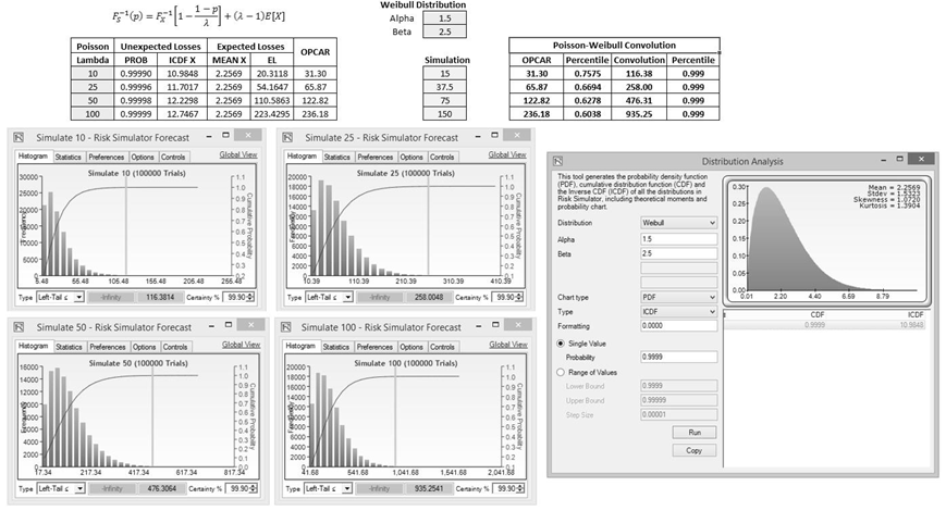
Figure TN.14: Comparing Basel OPCAR, Monte Carlo Risk Simulation, and the Convolution Algorithm
Theory
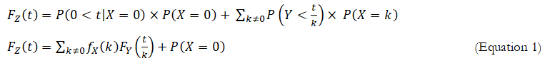
Let X, Y, and Z be real-valued random variables whereby X and Y are independently distributed with no correlations. Further, we define , ![]() as their corresponding CDFs, and fX, fY, fZ are their corresponding PDFs. Next, we assume that X is a random variable denoting the Frequency of a certain type of operational risk occurring and is further assumed to have a discrete Poisson distribution. Y is a random variable denoting the Severity of the risk (e.g., monetary value or some other economic value) and can be distributed from among a group of continuous distributions (e.g., Fréchet, Gamma, Log Logistic, Lognormal, Pareto, Weibull, etc.). Therefore, Frequency × Severity equals the Total Risk Losses, which we define as Z, where Z = X × Y.
as their corresponding CDFs, and fX, fY, fZ are their corresponding PDFs. Next, we assume that X is a random variable denoting the Frequency of a certain type of operational risk occurring and is further assumed to have a discrete Poisson distribution. Y is a random variable denoting the Severity of the risk (e.g., monetary value or some other economic value) and can be distributed from among a group of continuous distributions (e.g., Fréchet, Gamma, Log Logistic, Lognormal, Pareto, Weibull, etc.). Therefore, Frequency × Severity equals the Total Risk Losses, which we define as Z, where Z = X × Y.
Then the Total Loss formula, which is also sometimes known as the Single Loss Approximation (SLA) model, yields:
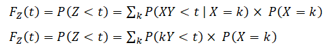
where the term with X=0 is treated separately:
(Equation 1)
The next step is the selection of the number of summands in Equation 1. As previously assumed,![]() is a Poisson distribution where
is a Poisson distribution where ![]()
and the rate of convergence in the series depends solely on the rate of convergence to 0 of
![]()
and does not depend on t, whereas the second multiplier![]()
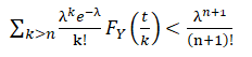
Therefore, for all values of t and an arbitrary δ > 0 there is value of n such that:
![]()
In our case, δ can be set, for example, to 1/1000. Thus, instead of solving the quantile equation for ![]() with an infinite series, on the left-hand side of the equation we have:
with an infinite series, on the left-hand side of the equation we have:
![]()
We can then solve the equation:
![]()
with only n summands.
For example, if we choose p = 0.95, δ =1/1000, and n such that Equation 2 takes place, then the solution ![]() of Equation 4 is such that:
of Equation 4 is such that:![]()
In other words, a quantile found from Equation 4 is almost the true value, with a resulting error precision in the probability of less than 0.1%.
The only outstanding issue that remains is to find an estimate for n given any level of δ. We have:
![]()
The exponential series ![]()
in Equation 6 is bounded by![]()
by applying Taylor’s Expansion Theorem, with the remainder of the function left for higher exponential function expansions. By substituting the upper bound for ![]()
in Equation 6, we have:
Now we need to find the lower bound in n for the solution of the inequality: Consider the following two cases:
- If λ≤1, then
 Consequently, we can solve the inequality
  Since
Since grows quickly, we can simply take n > – ln δ. For example, for
 it is sufficient to set n=7 to satisfy Equation 8.
 - If λ>1, then, in this case, using the same bounds for the factorial, we can choose n such that:

To make the second multiplier greater than 1, we will need to choose![]()
Approximation to the solution of the equation![]() for a quantile value
for a quantile value
From the previous considerations, we found that instead of solving![]() for t,we can solve
for t,we can solve ![]() with n set at the level indicated above. The value for
with n set at the level indicated above. The value for ![]() resulting from such a substitution will satisfy the inequality
resulting from such a substitution will satisfy the inequality![]()
Solution of the equation ![]() given n and δ.
given n and δ.
By moving t to the left one unit at a time, we can find the first occurrence of the event t = a such that![]() Similarly, moving t to the right we can find b such that
Similarly, moving t to the right we can find b such that![]() Now we can use a simple Bisection Method or other search algorithms to find the optimal solution
Now we can use a simple Bisection Method or other search algorithms to find the optimal solution
to ![]()
EMPIRICAL RESULTS: CONVOLUTION VERSUS MONTE CARLO RISK SIMULATION FOR OPCAR
Based on the explanations and algorithms outlined above, the convolution approximation models are run, and the results are compared with Monte Carlo risk simulation outputs. These comparisons will serve as empirical evidence of the applicability of both approaches.
Figure TN.15 shows the 10 most commonly used Severity distributions, namely, Exponential, Fréchet, Gamma, Logistic, Log Logistic, Lognormal (Arithmetic and Logarithmic inputs), Gumbel, Pareto, and Weibull. The Frequency of risk occurrences is set as Poisson, with Lambda (λ) or average frequency rate per period as its input. The input parameters for the 10 Severity distributions are typically Alpha (α) and Beta (β), except for the Exponential distribution that uses a rate parameter, Rho (ρ), and Lognormal distribution that requires the mean (μ) and standard deviation (σ) as inputs. For the first empirical test, we set λ= 10, α = 1.5, β = 2.5, ρ = 0.01, μ = 1.8, and σ = 0.5 for the Poisson frequency and 10 severity distributions. The Convolution Model row in Figure TN.15 was computed using the algorithms outlined above, and a set of Monte Carlo risk simulation assumptions were set with the same input parameters and simulated 100,000 trials with a prespecified seed value. The results from the simulation were pasted back into the model under the Simulated Results row and the Convolution Model was calculated based on these simulated outputs. Figure TN.15 shows 5 sets of simulation percentiles: 99.9%, 99.0%, 95.0%, 90.0%, and 50.0%. As can be seen, all of the simulation results and the convolution results on average agree to approximately within ±0.2%.
Figure TN.16 shows another empirical test whereby we select one specific distribution; in the illustration, we used the Poisson–Weibull compound function. The alpha and beta parameters in Weibull were changed, in concert with the Poisson’s lambda input. The first four columns show alpha and beta being held steady while changing the lambda parameter, whereas the last six columns show the same lambda with different alpha and beta input values (increasing alpha with beta constant and increasing beta with alpha constant). When the simulation results and the convolution results were compared, on average, they agree to approximately within ±0.2%.
Figure TN.17 shows the Credit, Market, Operational, and Liquidity (CMOL) risk software’s operational risk module and how the simulation results agree with the convolution model. The CMOL software uses the algorithms as described above. The CMOL software settings are 100,000 Simulation Trials with a Seed Value of 1 with an OPCAR set to 99.90%.
Figures TN.18–TN.21 show additional empirical tests where all 10 severity distributions were perturbed, convoluted, and compared with the simulation results. The results agree on average around ±0.3%.
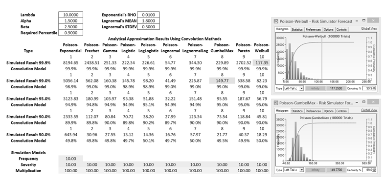
Figure TN.15: Comparing Convolution to Simulation Results I
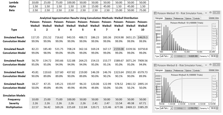
Figure TN.16: Comparing Convolution to Simulation Results II
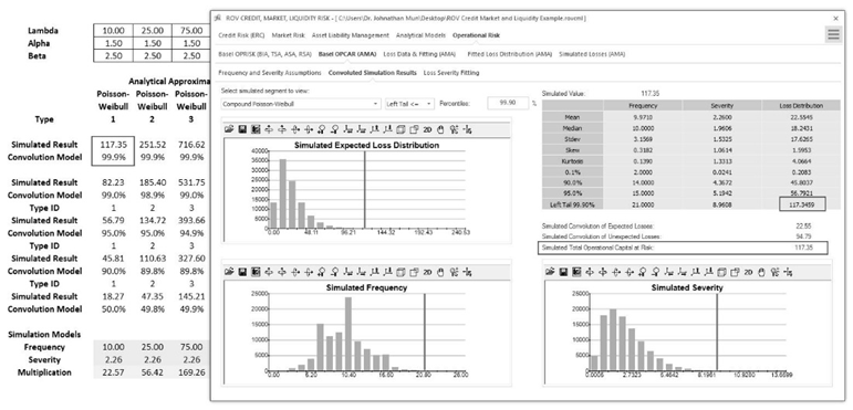
Figure TN.17: Comparing Convolution to Simulation Results III
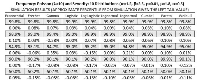
Figure TN.18: Empirical Results 1: Small Value Inputs
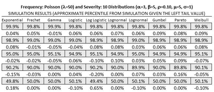
Figure TN.19: Empirical Results 2: Average Value Inputs
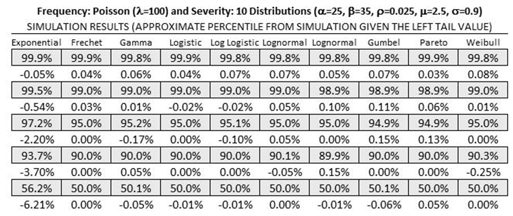
Figure TN.20: Empirical Results 3: Medium Value Inputs
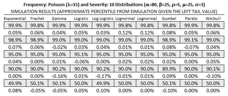
Figure TN.21: Empirical Results 4: High Value Inputs
HIGH LAMBDA AND LOW LAMBDA LIMITATIONS
As seen in Equation 4, we have the![]() convolution model. The results are accurate to as many decimal-points precision as desired as long as n is sufficiently large, but this would mean that the convolution model is potentially mathematically intractable. When λ and k are high (the value k depends on the Poisson rate λ),such as λ = 10,000, the summand cannot be easily computed. For instance, Microsoft Excel 2013 can only compute up to a factorial of 170! where 171! and above returns the #NUM! error. Banks whose operational risks have large λ rate values (extremely high frequency of risk events when all risk types are lumped together into a comprehensive frequency count) have several options: Create a breakdown of the various risk types (broken down by risk categories, by department, by division, etc.) such that the λ is more manageable; use a continuous distribution approximation as shown below; or use Monte Carlo risk simulation techniques, where large λ values will not pose a problem whatsoever.
convolution model. The results are accurate to as many decimal-points precision as desired as long as n is sufficiently large, but this would mean that the convolution model is potentially mathematically intractable. When λ and k are high (the value k depends on the Poisson rate λ),such as λ = 10,000, the summand cannot be easily computed. For instance, Microsoft Excel 2013 can only compute up to a factorial of 170! where 171! and above returns the #NUM! error. Banks whose operational risks have large λ rate values (extremely high frequency of risk events when all risk types are lumped together into a comprehensive frequency count) have several options: Create a breakdown of the various risk types (broken down by risk categories, by department, by division, etc.) such that the λ is more manageable; use a continuous distribution approximation as shown below; or use Monte Carlo risk simulation techniques, where large λ values will not pose a problem whatsoever.
Poisson distributions with large λ values approach the Normal distribution, and we can use this fact to generate an approximation model for the convolution method. The actual deviation between Poisson and Normal approximation can be estimated by the Berry–Esseen inequality. For a more accurate and order of magnitude tighter estimation we can use the Wilson–Hilferty approximation instead. For the large lambda situation, we can compute the CDF of the compound of two continuous distributions whose PDFs are defined as ƒ(x) defined on the positive interval of (a,b) for the random variable X, and g(y) defined on the positive interval of (c,d), for the random variable Y. In other words, we have 0 < a < b < ∞ and 0 < c < d < ∞. The joint distribution Z = XY has the following characteristics:
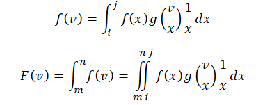
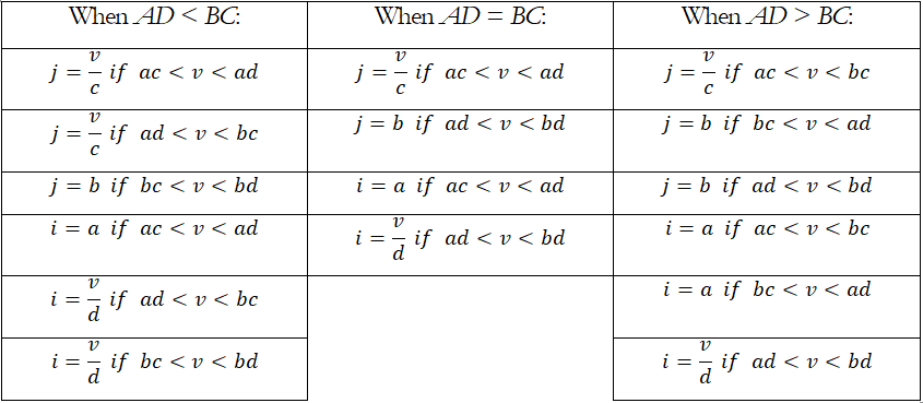
The integration can be applied analytically using numerical integration methods, but the results will critically depend on the integration range of x and v. The values of a, b, c, d can be computed by taking the inverse CDF of the distributions at 0.01% and 99.99% respectively (e.g., in the Normal distribution, this allows us to obtain real values instead of relying on the theoretical tails of -∞ and +∞). The following table summarizes the integration ranges:
To obtain the values of m and n, we can first run a Monte Carlo Risk Simulation of the two independent distributions, then multiply them to obtain the joint distribution, and from this joint distribution, we obtain the left tail 0.01% value, and set this as m. The value of n is the left tail VaR% (e.g., 99.95%) value. The second integral when run based on this range, will return the CDF percentile of the OPCAR VaR. Alternatively, as previously described, the Bisection Method can be used to obtain the lowest value of m by performing iterative searches such that the CDF returns valid results at 0.01% and then a second search is performed to identify the upper range or n, where the resulting n that makes the integral equal to the user-specified VaR%, i.e., the OPCAR value.
Finally, for low lambda values, the algorithm still runs but will be a lot less accurate. Recall in Equation 2 that![]()
where δ signifies the level of error precision (the lower the value, the higher the precision and accuracy of the results). The problem is, with low λ values, both k and n, which depend on λ, will also be low. This means that in the summand there would be an insufficient number of integer intervals, making the summation function less accurate. For best results, λ should be between 5 and 100.
CAVEATS, CONCLUSIONS, AND RECOMMENDATIONS
Based on the theory, application, and empirical evidence above, one can conclude that the convolution of Frequency × Severity independent stochastic random probability distributions can be modeled using the algorithms outlined above as well as using Monte Carlo simulation methods. On average, the results from these two methods tend to converge with some slight percentage variation due to randomness in the simulation process and the precision depending on the number of intervals in the summand or numerical integration techniques employed.
However, as noted, the algorithms described above are only applicable when the lambda parameter 5 ≤ λ ≤ 100, else the approximation using numerical integration approach is required.
In contrast, Monte Carlo risk simulation methods are applicable in any realistic lambda situation (in simulation, a high lambda condition can be treated by using a Normal distribution). As both the numerical method and simulation approach tend to the same results, and seeing that simulation can be readily and easily applied in CMOL and using Risk Simulator, we recommend using simulation methodologies for the sake of simplicity. The Basel Committee has, throughout its Basel II-III requirements and recommendations, sought for simplicity so as not to burden the banks with added complexity, and yet it still requires sufficient rigor and substantiated theory. Therefore, Monte Carlo risk simulation methods are the recommended path when it comes to modeling OPCAR.