- Related AI/ML Methods: Multivariate Discriminant Analysis, Segmentation Clustering
- Related Traditional Methods: Linear Discriminant Analysis, Segmentation Clustering
Support Vector Machines (SVM) is a class of supervised machine learning algorithms used for classification. The term “machine” in SVM might be a misnomer in that it is only a vestige of the term “machine learning.” SVM methods are simpler to implement and run than complex neural network algorithms. In supervised learning, we typically start with a set of training data. The algorithm is trained using this dataset (i.e., the parameters are optimized and identified), and then the same model parameters are applied to the testing set, or to a new dataset never before seen by the algorithm. The training dataset comprises m data points, placed as rows in the data grid (Figure 9.62), where there is an outcome or dependent variable ![]() , followed by one or more independent predictors
, followed by one or more independent predictors ![]() for
for ![]() . Each of the dependent (also known as predictor or feature) variables has n dimensions (number of columns). In contrast, there is only a single
. Each of the dependent (also known as predictor or feature) variables has n dimensions (number of columns). In contrast, there is only a single ![]() variable, with a binary outcome (e.g., 1 and 0, or 1 and 2, indicating if an item is in or out of a group). Note that the training set can also be used as the testing set, and the results will typically yield a high level of segregation accuracy. However, in practice, we typically use a smaller subset of the testing dataset as the training dataset and unleash the optimized algorithm on the remaining testing set. One of the few limiting caveats of SVM methods is a requirement that there exists some n-dimensional hyperplane that separates the data.
variable, with a binary outcome (e.g., 1 and 0, or 1 and 2, indicating if an item is in or out of a group). Note that the training set can also be used as the testing set, and the results will typically yield a high level of segregation accuracy. However, in practice, we typically use a smaller subset of the testing dataset as the training dataset and unleash the optimized algorithm on the remaining testing set. One of the few limiting caveats of SVM methods is a requirement that there exists some n-dimensional hyperplane that separates the data.
The hyperplane is defined by an equation ![]() , which completely separates the training dataset into two groups. The parameters w (the normal vector to the hyperplane) and b (an offset parameter such as a virtual intercept) can be scaled as needed, to adjust the forecast back into the original two groups. Applying some analytical geometry, we see that the parameters are best fitted by applying an internal optimization routine to minimize
, which completely separates the training dataset into two groups. The parameters w (the normal vector to the hyperplane) and b (an offset parameter such as a virtual intercept) can be scaled as needed, to adjust the forecast back into the original two groups. Applying some analytical geometry, we see that the parameters are best fitted by applying an internal optimization routine to minimize ![]() which reduces to a Lagrangian problem where we maximize the likelihood of
which reduces to a Lagrangian problem where we maximize the likelihood of ![]() where all parameters are positive.
where all parameters are positive.
Finally, SVM algorithms are best used in conjunction with a kernel density estimator, and the three most commonly used are the Gaussian, Linear, and Polynomial kernels. Try each of these approaches and see which fits the data the best by reviewing the accuracy of the results.
- Gaussian SVM. Applies a normal kernel estimator exp
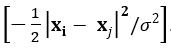 .
. - Linear SVM. Applies a standard linear kernel estimator
 .
. - Polynomial SVM. Applies a polynomial (e.g., quadratic nonlinear programming) kernel density estimator such as
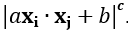 .
.
Figure 9.62 illustrates the SVM supervised model. The same procedure applies to all three SVM subclasses. To get started, we use an example dataset where the weights and sizes of 40 fruits were measured. These fruits were either apples or oranges. Recall that SVMs are best used for separations into two groups. The data grid shows VAR408 with the alphanumeric category of the dependent or classified variable (apples or oranges). However, the SVM algorithms require numerical inputs, hence, the dependent groupings have been coded to a numerical value of 1 and 2 in VAR407 (bivariate numerical categories). VAR405 and VAR406 are the predictors or features set (the weights and sizes of the fruits) that we will use as the training set to calibrate and fit the model. These are the first two sets of inputs in the model. Note that we have VAR407 entered in the first row as the training dependent variable and in the second row, VAR405; VAR406 as the training independent variables (predictor feature set). To get started, we use the default Sigma, Lambda, and Omega values of 2, 1000, and 0.5. Depending on the SVM subclass, only some or all three of these will be used. Start with the defaults and change as required. The main variable that impacts the results is the Omega, which is a value between 0 and 1. If you set the Calibrate Option to 1, it will test various Omega values and shows the accuracy levels of each. Select the Omega value with the highest accuracy and rerun the model. You can access the dataset and input parameters in BizStats by loading the default example. The following illustrates the required input parameters and examples:
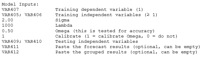
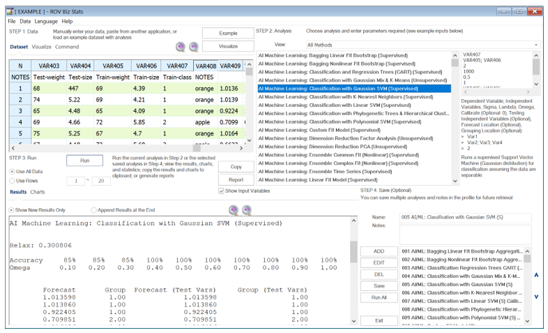
Figure 9.62: AI/ML Classification with Support Vector Machines (SVM)
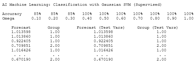
The results provide a series of forecast values and forecast groups for the training set as well as for the testing dataset, showing the numerical segmentation results and the final resulting groups. Note that the example results indicate relatively high goodness of fit to the training dataset at 95% fit. This fit applies to the training dataset and assuming the same data structure holds, the testing dataset should also have a fit that is close to this result. Typically, only the testing dataset’s forecast values and grouping membership are important to the user; hence, you can optionally enter the location in the data grid to save the results, for example, VAR411 and VAR412. If these inputs are left empty, the results will not be saved in the data grid, and they will only be available in the results area.