File Name: Optimization – Discrete Project Selection
Location: Modeling Toolkit | Optimization | Discrete Project Selection
Brief Description: Illustrates how to run an optimization on discrete integer decision variables in project selection in order to choose the best projects in a portfolio given a large variety of project options, subject to risk, return, budget, and other constraints
Requirements: Modeling Toolkit, Risk Simulator
This model shows 12 different projects with different risk and return characteristics. The idea here is to find the best portfolio allocation such that the portfolio’s total strategic returns are maximized. That is, the model is used to find the best project mix in the portfolio that maximizes the total returns after considering the risks and returns of each project, subject to the constraints of the number of projects and the budget. Figure 95.1 illustrates the model.
Objective: Maximize Total Portfolio Returns (C17) or Sharpe Ratio returns to risk
ratio (C19)
Decision Variables: Allocation or Go/No-Go Decision (I4:I15)
Restrictions on Decision Variables: Binary decision variables (0 or 1)
Constraints: Total Cost (D17) is less than $5000 and less than or equal to 6 projects
selected (I17)
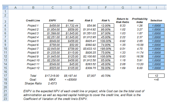
Figure 95.1: Discrete project selection model
Running an Optimization
To run this preset model, simply run the optimization (Risk Simulator | Optimization | Run Optimization), or for practice, set up the model yourself:
- Start a new profile(Risk Simulator | New Profile) and give it a name.
- In this example, all the allocations are required to be binary (0 or 1) values, so first select cell I4 and make this a decision variable in the Integer Optimization worksheet and select cell I4 and define it as a decision variable (Risk Simulator | Optimization | Decision Variables or click on the Define Decision icon) and make it a Binary Variable. This setting automatically sets the minimum to 0 and maximum to 1 and can only take on a value of 0 or 1. Then use the Risk Simulator Copy on cell I4, select cells I5 to I15, and use Risk Simulator’s Paste (Risk Simulator | Copy Parameter and Risk Simulator | Paste Parameter or use the Risk Simulator copy and paste icons, NOT the Excel copy/paste).
- Next, set up the optimization’s constraints by selecting Risk Simulator | Optimization | Constraints and selecting ADD. Then link to cell D17, and make it <= 5000, and select ADD one more time and click on the link icon and point to cell I17 and set it to <=6.
- Select cell C19, the objective to be maximized, and select Risk Simulator | Optimization | Set Objective and then select Risk Simulator | Optimization | Run Optimization. Review the different tabs to make sure that all the required inputs in steps 2 and 3 above are correct.
- You may now select the optimization method of choice and click OK to run the optimization.
Note: Remember that if you are to run either a dynamic or stochastic optimization routine, make sure that you first have assumptions defined in the model. That is, make sure that some of the cells in C4:C15 are assumptions. The suggestion for this model is to run a Discrete Optimization.
Viewing and Interpreting Forecast Results
In addition, you can create a Markowitz Efficient Frontier by running the optimization, then resetting the budget and number of projects constraints to a higher level, and rerunning the optimization. You can do this several times to obtain the Risk-Return efficient frontier. For a more detailed example, see Chapter 100 on the military portfolio and efficient frontier models.
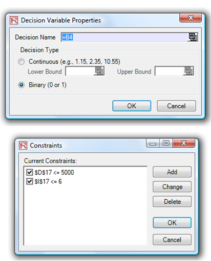
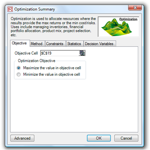
Figure 95.2: Setting up the optimization process