File Name: Simulation – Best Surgical Team
Location: Modeling Toolkit | Risk Simulator | Best Surgical Team
Brief Description: Illustrates how to use Risk Simulator for simulating the chances of a successful surgery and understanding the distribution of successes, using the Distribution Analysis tool to compute the CDF and ICDF of the population distribution, and using Bootstrap Simulation to obtain the statistical confidence of success rates
Requirements: Modeling Toolkit, Risk Simulator
In this model, we analyze six hospitals and look at their respective successes and failures when it comes to a specific type of surgical procedure. This historical information is tabulated in the Model worksheet and is summarized in Figure 133.1.
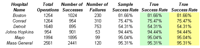
Figure 133.1: Historical surgical success rates
For instance, Boston General Hospital had 1,254 surgical cases of a specific nature within the past five years, and out of those cases, 1,024 were considered successful while 230 cases were not successful (based on predefined requirements for failures and successes). Therefore, the sample success rate is 81.66%. The problem is, this is only a small sample and is not indicative of the entire population (i.e., all possible outcomes). In this example, we simply assume that history repeats itself. Because there are dozens of surgeons performing the same surgery and the tenure of a surgeon extends multiple years, we assume this is adequate, and that any small changes in staffing do not necessarily create a significant change in the success rates. Otherwise, more data should be collected and multivariate regressions and other econometric modeling should be performed to determine if the composition of surgeons and other medical practitioners will contribute in a statistically significant way to the rates of success, and we use simulation as well as distributional and probabilistic models to predict the successful outcomes. In addition, jump-diffusion or new medical technology advances might also contribute to a higher success rate. The advent of these technologies and their corresponding contributions to success rates can be modeled using the custom distribution through solicitation from subject matter experts in the area. Nonetheless, for this example, we look at using historical data to forecast the potential current success rate and to determine the entire population’s distribution of success rates.
Monte Carlo Simulation
Success rates are distributed following a Beta distribution, where the alpha parameter is the number of successes in a sample, and the beta parameter is the number of failures. For instance, the Boston hospital’s distribution of success rates is a Beta (1024, 230). Using Risk Simulator’s set input assumption (Figure 133.2), you can see that the theoretical mean is 0.8166, equivalent to the sample success rate of 81.66% computed previously.
Just knowing the sample mean is insufficient. By using simulation, we can now reconstitute the entire population based on the sample success rate. For instance, running a simulation on the model yields the forecast results shown in Figures 133.3 and 133.4 for the Boston hospital.
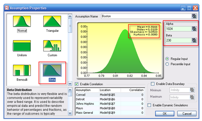
Figure 133.2: Set input assumption
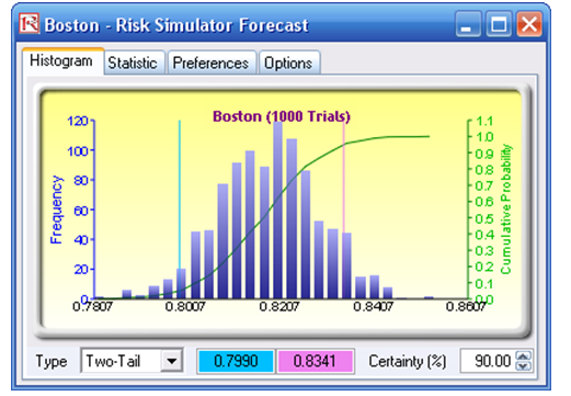
Figure 133.3: Boston hospital’s forecast output
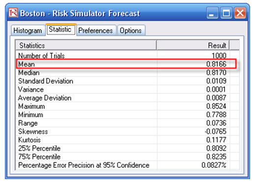
Figure 133.4: Boston hospital’s forecast statistics
After running 1,000 trials, the expected value is 81.66%. In addition, we now have a slew of statistics associated with the success rate at Boston. The theoretical success rate is between 77.88% and 85.24%, and is fairly symmetrical with a skew close to zero (Figure 133.4). Further, the 90% confidence puts the success rate at between 79.90% and 83.41% (Figure 133.3). You can now perform a comparison among all the hospitals surveyed and see which hospital is the safest place to get the procedure done.
Procedures for Running Monte Carlo Simulation
This model already has assumptions and forecasts predefined for you. To run the predefined model, simply:
- Go to the Model worksheet and click on Risk Simulator | Change Profile and select the Best Surgical Team profile.
- Click on the RUN icon or select Risk Simulator | Run Simulation.
- Select the forecast chart of your choice (e.g., Boston) and use the Two-Tail analysis. Type 90 in the Certainty box and hit TAB on the keyboard.
- You can enter in other certainty values and hit TAB to obtain other confidence results. Also, click on the Statistics tab to view the distributional statistics.
To recreate the model’s assumptions and forecasts, simply:
- Go to the Model worksheet and click on Risk Simulator | New Profile and give it a new profile name of your choice.
- Select cell G4 and click on Risk Simulator | Set Input Assumption. Select the BETA distribution and enter in the relevant parameters (e.g., type in 1024 for Alpha and 230 for Beta) and click OK. Repeat for the other cells in G5 to G9.
- Select H4 and click on Risk Simulator | Set Output Forecast and give it a relevant name (e.g., Boston), and repeat by setting the rest of the cells in H5 to H9 as forecast cells.
- Click on the RUN icon or select Risk Simulator | Run Simulation.
- Select the forecast chart of your choice (e.g., Boston) and use the Two-Tail analysis. Type 90 in the Certainty box and hit TAB on the keyboard.
- You can enter in other certainty values and hit TAB to obtain other confidence results. Also, click on the Statistics tab to view the distributional statistics.
Distribution Analysis
In addition, because we are now able to reconstitute the entire distribution, we can use the information to compute and see the various confidence levels and their corresponding success rates by using the Distribution Analysis tool. For instance, selecting the Beta distribution and entering the relevant input parameters, and choosing the cumulative distribution function (CDF), we can now see that, say, 81.5% success rate has a CDF of about 43.6% (Figure 133.5). This means that you have a 43.6% chance that the success rate is less than or equal to 81.5%, or that you have a 56.4% chance that your success rate will be at least 81.5%, and so forth. These values are theoretical values. An alternative approach is to use the forecast chart and compute the left-tail probability (CDF). Here we see the empirical results show that the probability of getting less than 81.5% success rate is 43.9% (Figure 133.6), close enough to the theoretical. Clearly, the theoretical results are more reliable and accurate. Nonetheless, the empirical results approach the theoretical when enough trials are run in the simulation.
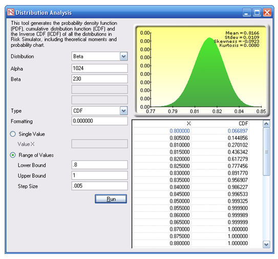
Figure 133.5: Distributional analysis tool
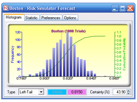
Figure 133.6: Empirical results
Conversely, you can compute the Inverse CDF or ICDF of the distribution. For instance, the 10% CDF shows an ICDF value of 80.24%, which means that you have a 10% chance of getting a success rate below or equal to 80.24% or that, from a more positive point of view, you have a 90% chance that the success rate is at least 80.24% (Figure 133.7).
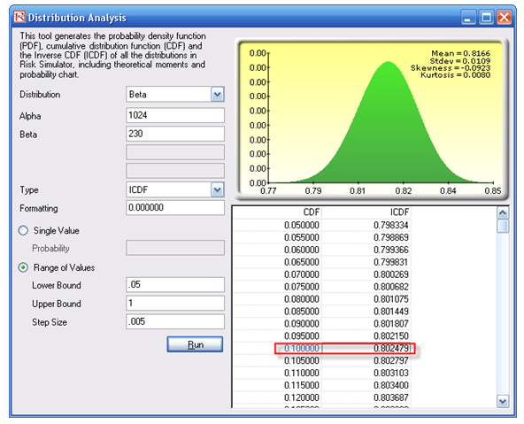
Figure 133.7: CDF and ICDF of exact probabilities
Procedures for Running a Distribution Analysis
- Start the Distribution Analysis tool (click on Risk Simulator| Tools | Distribution Analysis).
- Select the Beta distribution and enter 1024 for Alpha and 230 for Beta parameters, and select CDF as the analysis Then, select Range of Values and enter 0.8 and 1 as the lower and upper bounds, with a step of 0.005, and click RUN.
- Now change the analysis type to ICDF and the bounds to between 05 and 1 with a step size of 0.005 and click RUN.
Bootstrap Simulation
A Bootstrap simulation can also be run on the resulting forecast. For instance, after running a simulation on the model, a bootstrap is run on the Boston hospital on its mean, maximum, and minimum values (Figure 133.8).
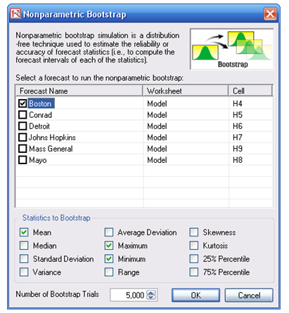
Figure 133.8: Bootstrap simulation tool
The results indicate that there is a 90% statistical confidence that the average success rate of the true population is between 81.6% and 81.7%, with the lowest or minimum success rate you can be assured of, at a 90% confidence, of between 77.8% and 78.5%. This means that 90 out of a 100 times a surgery is performed, or 90% confidence, the lowest and most conservative success rate is between 77.8% and 78.5%. For an additional exercise, change the confidence levels to 95% and 99% and analyze the results. Repeat for all other hospitals.
Procedures for Bootstrap Simulation
To run a bootstrap simulation, follow the steps below:
- Run a simulation based on the steps outlined above. You cannot run a bootstrap unless you first run a simulation.
- Click on Risk Simulator | Analytical Tools | Nonparametric Bootstrap and select the hospital of your choice (e.g., Boston), and then select the statistics of your choice (e.g., mean, maximum, minimum), enter 5000 as the number of bootstrap trials, and click OK.
- Select Two-Tail on the statistics forecast chart of your choice (e.g., Mean), type in 90 in the Certainty box, and hit TAB on the keyboard to obtain the 90% statistical confidence interval of that statistic. Repeat on other statistics or use different tails and confidence levels (Figures 133.9 and 133.10).

Figure 133.9: Bootstrapped mean values
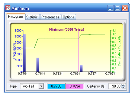
Figure 133.10: Bootstrapped minimum values