Single Moving Average
The single moving average is applicable when time-series data with no trend and no seasonality exist. The approach simply uses an average of the actual historical data to project future outcomes. This average is applied consistently moving forward, hence the term moving average.
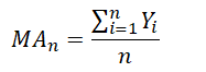
The value of the moving average (MA) for a specific length (n) is simply the summation of actual historical data (Y) arranged and indexed in time sequence (i):
An example computation of a 3-month single moving average is seen in Figure 12.2. Here we see that there are 39 months of actual historical data and a 3-month moving average is computed. Additional columns of calculations also exist in the example, calculations that are required to estimate the error of measurements in using this moving-average approach. These errors are important as they can be compared across multiple moving averages (i.e., 3-month, 4-month, 5-month, and so forth), as well as other time-series models (e.g., single moving average, seasonal additive model, and so forth) to find the best fit that minimizes these errors. Figures 12.3, 12.4, and 12.5 show the calculations used in the moving average model. Notice that the forecast-fit value in period 4 of 198.12 is a 3-month average of the prior three periods (months 1 through 3). The forecast-fit value for period 5 would then be the 3-month average of months 2 through 4. This process is repeated moving forward until month 40 (Figure 12.4) where every month after that, the forecast is fixed at 664.97. Clearly, this approach is not suitable if there is a trend (upward or downward over time) or if there is seasonality. Thus, error estimation is important when choosing the optimal time-series forecast model. Figure 12.3 illustrates a few additional columns of calculations required for estimating the forecast errors. The values from these columns are used in Figure 12.5’s error estimation.
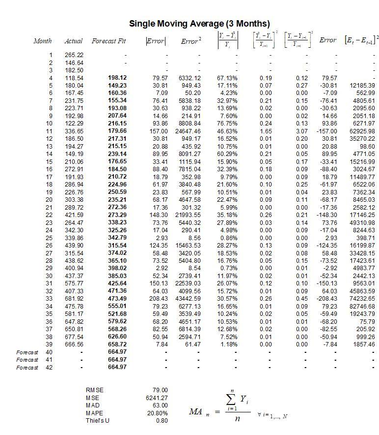
Figure 12.2: Single Moving Average (3 Months)
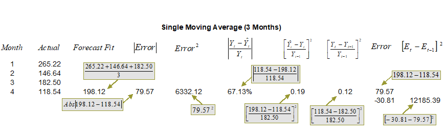
Figure 12.3: Calculating Single Moving Average
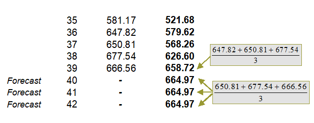
Figure 12.4: Forecasting with a Single Moving Average
Error Estimation (RMSE, MSE, MAD, MAPE, Theil’s U)
Several different types of errors can be calculated for time-series forecast methods, including the mean squared error (MSE), root mean squared error (RMSE), mean absolute deviation (MAD), and mean absolute percent error (MAPE).
The MSE is an absolute error measure that squares the errors (the difference between the actual historical data and the forecast-fitted data predicted by the model) to keep the positive and negative errors from canceling each other out. This measure also tends to exaggerate large errors by weighting the large errors more heavily than smaller errors by squaring them, which can help when comparing different time-series models. The MSE is calculated by simply taking the average of the Error2 column in Figure 12.1. RMSE is the square root of MSE and is the most popular error measure, also known as the quadratic loss function. RMSE can be defined as the average of the absolute values of the forecast errors and is highly appropriate when the cost of the forecast errors is proportional to the absolute size of the forecast error.
The MAD is an error statistic that averages the distance (absolute value of the difference between the actual historical data and the forecast-fitted data predicted by the model) between each pair of actual and fitted forecast data points. MAD is calculated by taking the average of the |Error| column in Figure 12.1, and is most appropriate when the cost of forecast errors is proportional to the absolute size of the forecast errors.
The MAPE is a relative error statistic measured as an average percent error of the historical data points and is most appropriate when the cost of the forecast error is more closely related to the percentage error than the numerical size of the error. This error estimate is calculated by taking the average of the![]() column in Figure 12.1, where Yt is the historical data at time t, while
column in Figure 12.1, where Yt is the historical data at time t, while![]() is the fitted or predicted data point at time t using this time-series method. Finally, an associated measure is the Theil’s U statistic, which measures the naivety of the model’s forecast. That is, if the Theil’s U statistic is less than 1.0, then the forecast method used provides an estimate that is statistically better than guessing. Figure 12.5 provides the mathematical details of each error estimate.
is the fitted or predicted data point at time t using this time-series method. Finally, an associated measure is the Theil’s U statistic, which measures the naivety of the model’s forecast. That is, if the Theil’s U statistic is less than 1.0, then the forecast method used provides an estimate that is statistically better than guessing. Figure 12.5 provides the mathematical details of each error estimate.
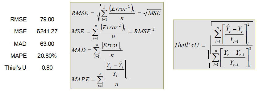
Figure 12.5: Error Estimation
Single Exponential Smoothing
The second approach to use when no discernable trend or seasonality exists is the single exponential-smoothing method. This method weights past data with exponentially decreasing weights going into the past; that is, the more recent the data value, the greater its weight. This weighting largely overcomes the limitations of moving averages or percentage-change models. The weight used is termed the alpha measure. The method is illustrated in Figures 12.6 and 12.7 and uses the following model:![]() where the exponential smoothing forecast (ESFt) at time t is a weighted average between the actual value of one period in the past (Yt-1) and the last period’s forecast (ESFt-1), weighted by the alpha parameter (α).
where the exponential smoothing forecast (ESFt) at time t is a weighted average between the actual value of one period in the past (Yt-1) and the last period’s forecast (ESFt-1), weighted by the alpha parameter (α).
Figure 12.7 shows an example of the computation. Notice that the first forecast-fitted value for month 2 or![]() is always the previous month’s actual value (Y1). The mathematical equation gets used only at month 3 or starting from the second forecast-fitted period.
is always the previous month’s actual value (Y1). The mathematical equation gets used only at month 3 or starting from the second forecast-fitted period.
The following are some sample calculations:
Forecast Fit for period 2 = Actual value in period 1 or 265.22
Forecast Fit for period 3 = 0.1 × 146.64 + (1 – 0.1) × 265.22 = 253.36
Forecast Fit for period 4 = 0.1 × 182.50 + (1 – 0.1) × 253.36 = 246.28
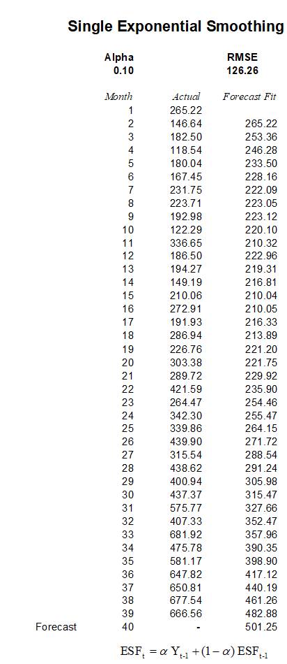
Figure 12.6: Single Exponential Smoothing
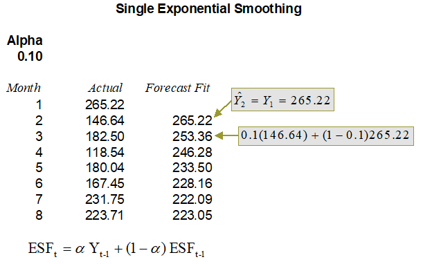
Figure 12.7: Calculating Single Exponential Smoothing
Optimizing Forecasting Parameters
Clearly, in the single exponential-smoothing method, the alpha parameter was arbitrarily chosen as 0.10. In fact, the optimal alpha has to be obtained for the model to provide a good forecast. Using the model in Figure 12.6, Excel’s Solver add-in package is applied to find the optimal alpha parameter that minimizes the forecast errors. Figure 12.8 illustrates Excel’s Solver add-in dialog box, where the target cell is set to the RMSE as the objective to be minimized by methodically changing the alpha parameter. As alpha should only be allowed to vary between 0.00 and 1.00 (because alpha is a weight given to the historical data and past period forecasts, and weights can never be less than zero or greater than one), additional constraints are also set up. The resulting optimal alpha value that minimizes forecast errors calculated by Solver is 0.4476. Therefore, entering this alpha value into the model will yield the best forecast values that minimize the errors. Risk Simulator’s time-series forecast module takes care of finding the optimal alpha level automatically as well as allows the integration of risk simulation parameters (see the previous chapters for details), but we show the manual approach here using Solver as an illustrative example.
Throughout this chapter, the alpha (α), beta (β), and gamma (ϒ) are the decision variables to be optimized, where each of these variables represents the weight of the time-series data’s Level (α), Trend (β), and Seasonality (ϒ), and each variable can take on any value between 0% and 100% (i.e., between 0 and 1, inclusive). The objective of the optimization is to minimize the forecast errors, which typically means minimizing RMSE. In other words, the minimum RMSE model implies the least amount of forecast errors or the highest level of accuracy achievable in the forecast model, or the best-fitting model given the historical data.
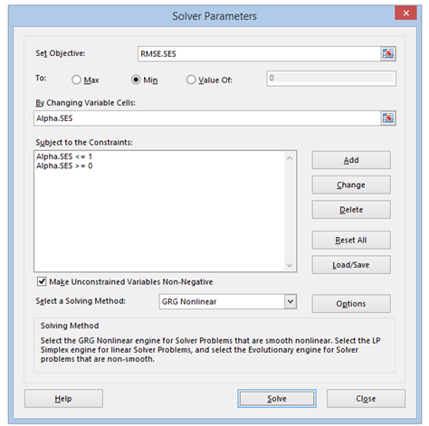
Figure 12.8: Optimizing Parameters in Single Exponential Smoothing