Figure 17.7 shows the efficient frontier constraints for optimization. You can get to this interface by clicking on the Efficient Frontier button after you have set some constraints. You can now make these constraints changing. That is, each of the constraints can be created to step through between some minimum and maximum value. As an example, the constraint in cell J17 <= 6 can be set to run between 4 and 8 (Figure 17.7). That is, five optimizations will be run, each with the following constraints: J17 <= 4, J17 <= 5, J17 <= 6, J17 <= 7, and J17 <= 8. The optimal results will then be plotted as an efficient frontier and the report will be generated (Figure 17.8).
Specifically, the following are the steps required to create a changing constraint:
- In an optimization model (i.e., a model with Objective, Decision Variables, and Constraints already set up), click on Risk Simulator | Optimization | Constraints and then click on Efficient Frontier.
- Select the constraint you want to change or step (e.g., J17), enter the parameters for Min, Max, and Step Size (Figure 17.7), and click ADD, then OK, and OK You should deselect the D17 <= 5000 constraint before running.
- Run Optimization as usual (Risk Simulator | Optimization | Run Optimization). You can choose static, dynamic, or stochastic. To get started, select the Static Optimization to run.
- The results will be shown as a user interface (Figure 17.8). Click on Create Report to generate a report worksheet with all the details of the optimization runs.
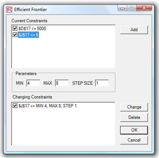
Figure 17.7: Generating Changing Constraints in an Efficient Frontier
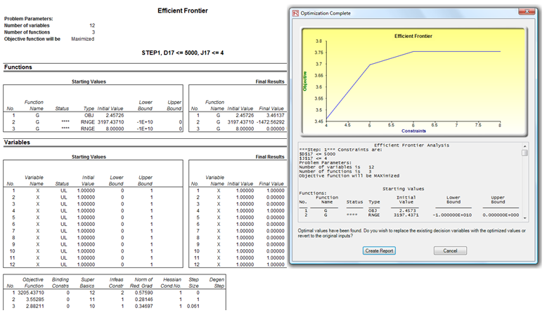
Figure 17.8: Efficient Frontier Results