The Risk Register section represents the center of the ERM world, and in the PEAT software, multiple Risk Registers can be created in a single file. That is, users are able to create multiple Risk Registers as seen in Figure 2.5, where we see three example registers: Project DGS728, CEO Presentation to the Board, and Project MMS5528. Each of these Risk Registers has multiple Risk Elements. These Risk Elements are shown at the bottom grid of the software. In Figure 2.5, the first four Risk Elements can be seen. Each Risk Element consists of a Risk Element Name, Acronym or Short Name, Causes of Risk, Consequences of Risk, Risk Mitigation Response, Action Plan, Active Status, Risk Manager Assignments, Risk Category, Risk Likelihood, Risk Impact, Key Risk Indicators, Risk Dates (Creation, Edit, and Due Dates), Diversifiable or Controllable Risk ($), Undiversifiable or Residual Risk ($), Mitigation Cost ($), Multiple Risk Controls (Control Names, Weights, and % Mitigation), and so forth, as illustrated in Figure 2.5.
A simple analogy for a Risk Register and its Risk Elements would be a checkbook. In a family (corporation), there might be several individuals each with their own checkbooks (Risk Register). In each checkbook, there will be a stack of checks. Each check can be seen as a Risk Element, where the recipient’s name, amount, date, and notes, can be entered (risk element name, causes, consequences, risk mitigation response, etc.). All Risk Elements roll up into a checkbook or Risk Register. A company can have one or more Risk Registers and each one can be created based on different projects, business units, investment initiatives, plants, facilities, and so on. So, each Risk Register contains multiple Risk Elements (e.g., the individual risks such as fire, fraud, IT downtime, human errors, accidents, and so forth, within each project, business unit, initiative, facility, etc.), shown as rows in the data grid (Figure 2.5).
Risk Category is also a required input and is based on the Risk Mapping previously performed, whereby selecting a specific Risk Category will automatically insert the inputted risk into all mapped relationships, as will be used later in the Risk Dashboards and risk reports.
Multiple Risk Registers can be created and saved here. However, the ERM file needs to be saved as well, using the File | Save menu. A single saved *.rovprojecon file can hold multiple Risk Registers, each with multiple Risk Elements.
Saving, Editing, Reporting, and Importing
To get started creating a new Risk Register, click on the New button in the Risk Register list window (top right corner of the software). Then, proceed to enter at least some sample data such as Risk Element Name and Acronym, select the Status, Risk Manager, Risk Category, and enter the Risk Likelihood and Risk Impact values. All other inputs are optional. Then, click on the Create New button to create a new Risk Element based on the information that was just entered. Once there is at least one Risk Element, you can now enter a name for the Risk Register. Type in a name and then click Save As to create and save the Risk Register. You can stop at this point or continue. To continue adding more Risk Elements, click on the name of the new Risk Register or any other Risk Register of choice, then click Edit to edit the Risk Register. Then, proceed to add more Risk Element information and click Create New to create each new Risk Element. When done adding Risk Elements, click on Save Edited and the Risk Register will be saved. When all data entry is done, do not forget to save the file using the menu File | Save or File | Save As, depending on what is required.
If data exists, clicking on Report will generate a report of all the Risk Registers. Each Excel worksheet will be its own Risk Register. A second report will also be generated, for all the Risk Controls. These reports can also be used as data input templates to Import into the software. Using the same files, replace the data with new data to import, save the Excel file and then, in the PEAT ERM software, click on the Import button to upload the Risk Registers.
Risk Element General Information
At a minimum, the required information for a Risk Element would be its name, acronym, likelihood and impact values, as well as the droplists for risk management assignment, and risk category. All other inputs are optional.
Risk Element Name should be descriptive, but its corresponding acronym or short name should be brief. The Acronym or Short Name should ideally fit into the data grid (8 characters or fewer).
Causes, Consequences, and Risk Mitigation Response are open-ended text input. These can be any length but would ideally be the length that can fit in the data grid, for the purposes of data clarity (around 80 characters or fewer).
A more detailed Action Plan such as an external document can be linked to a Risk Element by using the Browse button. The Notes icon beside the browse button can also be used to enter additional notes as required. This item is optional.
The three droplists need to be selected as these are considered required inputs. The Status droplist is defaulted to Active. Risk Elements that are subsequently deemed no longer applicable can either be Deleted or set as Inactive using this droplist. Making an item inactive will still keep it in the Risk Register for archiving purposes but its effects will not be computed in the Risk Dashboard later. The Assigned To droplist is where the relevant Risk Manager is selected. The list of Risk Managers was previously created in the Risk Settings | Risk Groups section. The same goes for the Risk Category droplist.
Risk Likelihood, Risk Impact, Risk Controls, Diversifiable Risk, Undiversifiable Risk, and Risk Mitigation
As previously mentioned, the Risk Element entries require a two-dimensional input of Risk Likelihood (L) or frequency of a risk event occurring and a Risk Impact (I) or the severity in terms of financial, economic, and non-economic effects of the risk. These likelihood and impact concepts are industry standards and used even in regulatory environments such as the Basel IV Accords (initiated by the Bank of International Settlements in Switzerland and accepted by most Central Banks around the world as regulatory reporting standards for operational risks). Alternate measures such as Vulnerability (V), Velocity (υ), and others can be used as well. (The case study in Chapter 4 on applying PEAT ERM at Eletrobrás in Brazil showcases one example of how Vulnerability measures are used.)
The uncertainties of repetitive events observed in enterprises’ operations over long periods of time can become predictable but usually not with absolute certainty. Such observances can be associated with mathematical functions that reflect the statistical properties of something likely to occur at a future time. The risk of an event occurring is connected to two parameters: The Risk Impact caused by an uncertain event and the probability, or Risk Likelihood, of an event occurring. Given some known probability of a risk event occurring, the higher the impact, the greater the risk. If the impact is zero, the risk will be zero even though the event has a high probability of occurring. The reverse argument is also true. If the probability of a risk event occurring is equal to zero, then the risk is zero (this is an environment of pure certainty), regardless of the magnitude of the impact.
Risks are also segregated into Diversifiable (risks that can be hedged, reduced, mitigated, or even completely eliminated) and Undiversifiable (these are residual or leftover risks that cannot be reduced any further). A simple example would be that of a fire risk. A manufacturing facility that has total assets of $1M may be able to hedge its fire risk by purchasing fire insurance and installing a state-of-the-art sprinkler system. These are two Risk Controls that may cost, say, $25,000 and $15,000 respectively. However, the total risk of $1M may not be completely reduced because if a fire does break out and the entire facility goes down in flames, the insurance may only cover 90% of the asset, as there is a $100,000 deductible. This $100,000 deductible is the undiversified risk, and the $900,000 would be the diversified risk.
So, the required inputs of Risk Likelihood and Risk Impact are also divided into Diversifiable Risk and Undiversifiable Risk. By construction, the diversifiable amount is greater than or equal to the undiversifiable amount. The data input in the four boxes are integers and are based on the range previously selected in the Risk Settings | Global Settings section where either 1–5 or 1–10 is selected. Figure 2.5 shows an example Risk Element with a 4 and 3 in terms of Risk Likelihood (based on a 1–10 range), then a 5 and 3 in terms of Risk Impact. Hence, the KRI would be 4 × 5 = 20 for the diversifiable risk and 3 × 3 = 9 for the undiversifiable risk. These KRIs are computed in the data grid and color coded based on the color scheme previously selected in the Global Settings section.
The Date Created and Date Updated are automatically set, whereas the Due Date can be set up as required, indicating by when a certain risk issue needs to be updated or resolved.
The optional section of Risk Controls can be entered if required. Using the examples above, Risk Control 1 can be fire insurance and the sprinkler system can be Risk Control 2. The % Weight can be entered such that the total equals 100%, indicating how much of a certain risk can be reduced with each control. The % Mitigation is between 0% and100% indicating how much of that control has been implemented. For instance, if only one quarter of the facility has sprinkler controls, then this would be entered as 25%. Additional rows of Risk Controls can be added or removed by clicking on the + and – icons. The total weight is also computed and by definition, must be 100%.
Diversifiable or Controllable Risk, Undiversifiable or Residual Risk, and Mitigation Cost are the optional monetary inputs in each Risk Element. Each one requires a Minimum, Most Likely, and Maximum input. Clearly, the minimum needs to be less than or equal to most likely, which is then less than or equal to the maximum value. Entering these ranges of values will allow Monte Carlo Risk Simulation to be run. For instance, the risks of a counterparty violating an existing contract may have financial impacts, where the minimal impact might be, say, $0 if the contract is still in force through the end of its term, to a most likely impact of $100,000 in anticipated delays and cost overruns by the counterparty, to a maximum of $300,000 if the counterparty becomes insolvent, resulting in lost business opportunities due to nonperformance of the counterparty.
The Mitigation Cost is the amount of money used to reduce the risk exposure of the specific Risk Element, for instance, the cost of obtaining a secondary subcontractor with prenegotiated terms whose contract becomes live only if the original contractor is not performing. Such risk mitigation methods tend to have a financial cost.
Finally, the computed Risk Exposure columns in the data grid deserve some added explanations. For example, in Figure 2.5, there are three Risk Controls with the following weights: 60%, 30%, and 10%, which add to 100%. The percent mitigation completed for these three controls is 100%, 0%, and 0%. This means the expected value of controls would be (60% × 100%) + (30% × 0%) + (10% × 0%) = 60%. This 60% completion value is automatically calculated and shown in the % OK column in the data grid. Also in the example, we see that the most likely diversifiable risk is $155,000 and the undiversifiable risk is $65,000. Since only 60% of the controllable diversifiable risk is executed, we have $65,000 + $155,000(1 – 60%) = $127,000 remaining, or the Current Risk level. As another example, if there are no controls or all controls have 0% Mitigation, it means there have been no risk controls, so, the current risk, in this case, would be $65,000 + $155,000 = $220,000. Alternatively, if all mitigations were 100%, all diversifiable risks have been controlled and all that is left is the undiversifiable risks or $65,000 + $155,000(1 – 100%) = $65,000 where current risk equals the undiversifiable residual risk.
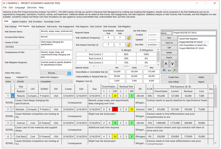
Figure 2.5: Risk Register