Figure 17.1 illustrates the sample continuous optimization model. The example here uses the example file located at Risk Simulator | Example Models | 11 Continuous Optimization. In this example, there are 10 distinct asset classes (e.g., different types of mutual funds, stocks, or assets) where the idea is to most efficiently and effectively allocate the portfolio holdings such that the best bang for the buck is obtained; that is, to generate the best portfolio returns possible given the risks inherent in each asset class. In order to truly understand the concept of optimization, we must delve more deeply into this sample model to see how the optimization process can best be applied.
The model shows the 10 asset classes and each asset class has its own set of annualized returns and annualized volatilities. These return and risk measures are annualized values such that they can be consistently compared across different asset classes. Returns are computed using the geometric average of the relative returns while the risks are computed using the logarithmic relative stock returns approach. See the appendix to this chapter for details on computing the annualized volatility and annualized returns on a stock or asset class.
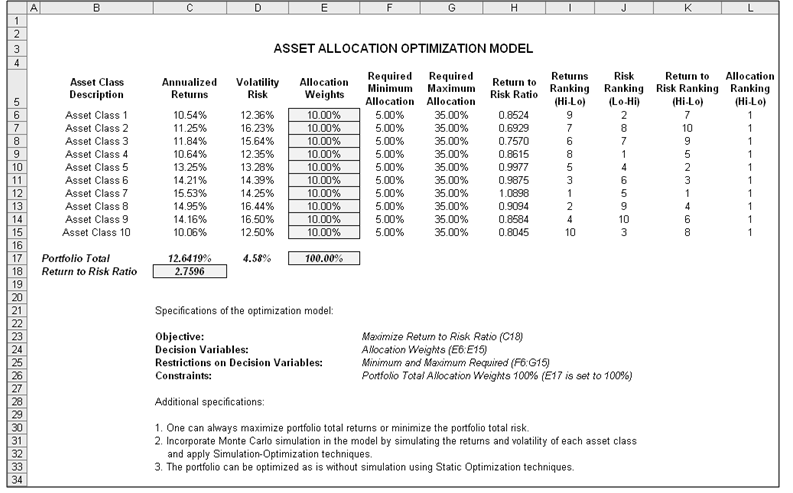
Figure 17.1: Continuous Optimization Model
The Allocation Weights in column E hold the decision variables, which are the variables that need to be tweaked and tested such that the total weight is constrained at 100% (cell E17). Typically, to start the optimization, we will set these cells to a uniform value, where in this case, cells E6 to E15 are set at 10% each. In addition, each decision variable may have specific restrictions in its allowed range. In this example, the lower and upper allocations allowed are 5% and 35%, as seen in columns F and G. This means that each asset class may have its own allocation boundaries. Next, column H shows the return to risk ratio, which is simply the return percentage divided by the risk percentage, where the higher this value, the higher the bang for the buck. The remaining model shows the individual asset class rankings by returns, risk, return to risk ratio, and allocation. In other words, these rankings show at a glance which asset class has the lowest risk, or the highest return, and so forth.
The portfolio’s total returns in cell C17 is SUMPRODUCT(C6:C15, E6:E15), that is, the sum of the allocation weights multiplied by the annualized returns for each asset class. In other words, we have ![]() where RP is the return on the portfolio, RA,B,C,D are the individual returns on the projects, and ωA,B,C,D are the respective weights or capital allocation across each project.
where RP is the return on the portfolio, RA,B,C,D are the individual returns on the projects, and ωA,B,C,D are the respective weights or capital allocation across each project.
In addition, the portfolio’s diversified risk in cell D17 is computed by taking ![]() Here, ρi,j are the respective cross-correlations between the asset classes. Hence, if the cross-correlations are negative, there are risk diversification effects, and the portfolio risk decreases. However, to simplify the computations here, we assume zero correlations among the asset classes through this portfolio risk computation, but assume the correlations when applying simulation on the returns as will be seen later. Therefore, instead of applying static correlations among these different asset returns, we apply the correlations in the simulation assumptions themselves, creating a more dynamic relationship among the simulated return values.
Here, ρi,j are the respective cross-correlations between the asset classes. Hence, if the cross-correlations are negative, there are risk diversification effects, and the portfolio risk decreases. However, to simplify the computations here, we assume zero correlations among the asset classes through this portfolio risk computation, but assume the correlations when applying simulation on the returns as will be seen later. Therefore, instead of applying static correlations among these different asset returns, we apply the correlations in the simulation assumptions themselves, creating a more dynamic relationship among the simulated return values.
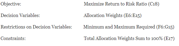
Finally, the return to risk ratio or Sharpe Ratio is computed for the portfolio. This value is seen in cell C18 and represents the objective to be maximized in this optimization exercise. To summarize, we have the following specifications in this example model:
Procedure
- Open the example file at Risk Simulator | Example Models | 11 Continuous Optimization and start a new profile by clicking on Risk Simulator | New Profile and provide it a name.
- The first step in optimization is to set the decision variables. Select cell E6 and set the first decision variable (Risk Simulator | Optimization | Set Decision) and click on the link icon to select the name cell (B6), as well as the lower bound and upper bound values at cells F6 and G6. Then, using Risk Simulator Copy, copy this cell E6 decision variable and paste the decision variable to the remaining cells in E7 to E15.
- The second step in optimization is to set the constraint. There is only one constraint here, that is, the total allocation in the portfolio must sum to 100%. So, click on Risk Simulator | Optimization | Constraints… and select ADD to add a new constraint. Then, select the cell E17 and make it equal (=) to 100%. Click OK when done.
- The final step in optimization is to set the objective function and start the optimization by selecting the objective cell C18 and Risk Simulator | Optimization | Set Objective and then run the optimization by selecting Risk Simulator | Optimization | Run Optimization and selecting the optimization of choice (Static Optimization, Dynamic Optimization, or Stochastic Optimization). To get started, select Static Optimization. Check to make sure the objective cell is set for C18 and select Maximize. You can now review the decision variables and constraints if required, or click OK to run the static optimization.
- Once the optimization is complete, you may select Revert to revert back to the original values of the decision variables as well as the objective, or select Replace to apply the optimized decision variables. Typically, Replace is chosen after the optimization is done.
Figure 17.2 shows the screenshots of the preceding procedural steps. You can add simulation assumptions on the model’s returns and risk (columns C and D) and apply the dynamic optimization and stochastic optimization for additional practice.
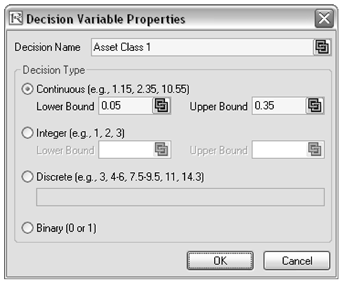
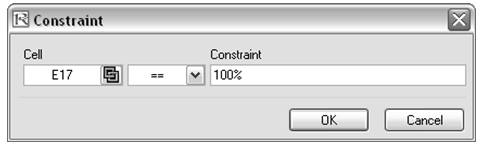
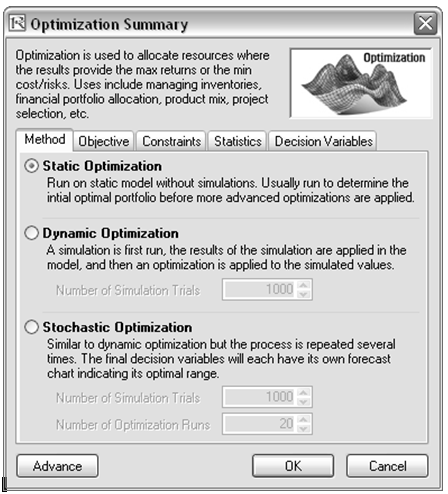
Figure 17.2: Running Continuous Optimization in Risk Simulator
Results Interpretation
The optimization’s final results are shown in Figure 17.3, where the optimal allocation of assets for the portfolio is seen in cells E6:E15. Given the restrictions of each asset fluctuating between 5% and 35%, and where the sum of the allocation must equal 100%, the allocation which maximizes the return to risk ratio is seen in Figure 17.3.
A few important things must be noted when reviewing the results and optimization procedures performed thus far:
- The correct way to run the optimization is to maximize the bang for the buck or returns to risk Sharpe Ratio as we have done.
- If instead, we maximized the total portfolio returns, the optimal allocation result is trivial and does not require optimization to obtain. That is, simply allocate 5% (the minimum allowed) to the lowest 8 assets, 35% (the maximum allowed) to the highest returning asset, and the remaining (25%) to the second-best returns asset. Optimization is not required. However, when allocating the portfolio this way, the risk is a lot higher as compared to when maximizing the returns to risk ratio, although the portfolio returns by themselves are higher.
- In contrast, one can minimize the total portfolio risk, but the returns will now be less.
The following table illustrates the results from the three different objectives being optimized:
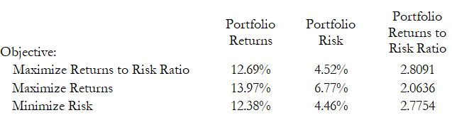
From the table, the best approach is to maximize the returns to risk ratio, that is, for the same amount of risk, this allocation provides the highest amount of return. Conversely, for the same amount of return, this allocation provides the lowest amount of risk possible. This approach of bang for the buck or returns to risk ratio is the cornerstone of the Markowitz efficient frontier in modern portfolio theory. That is, if we constrained the total portfolio risk levels and successively increased it over time we would obtain several efficient portfolio allocations for different risk characteristics. Thus, different efficient portfolio allocations can be obtained for different individuals with different risk preferences.
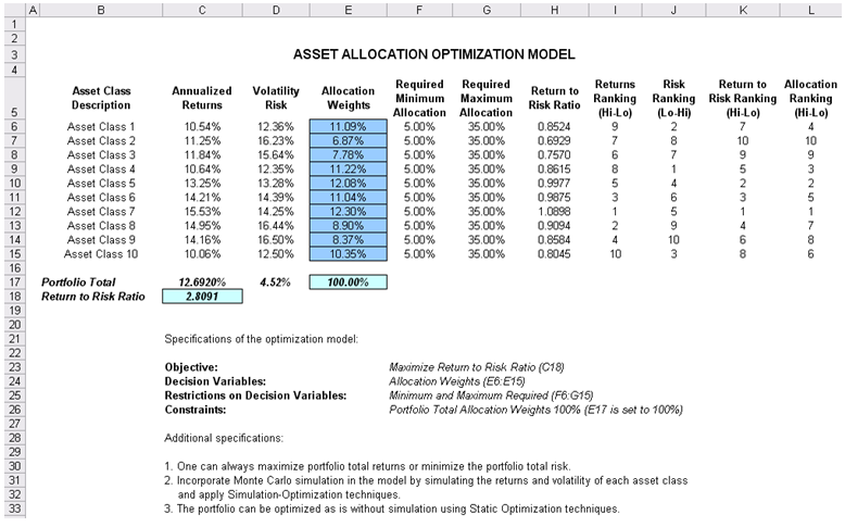
Figure 17.3: Continuous Optimization Results