File Name: Decision Analysis – Decision Tree Basics
Location: Modeling Toolkit | Decision Analysis | Decision Tree Basics
Brief Description: Shows how to create and value a simple decision tree as well as how to run a Monte Carlo simulation on a decision tree
Requirements: Modeling Toolkit, Risk Simulator
This model provides an illustration on the basics of creating and solving a decision tree. This forms the basis for the more complex model (see the Decision Tree with EVPI, Minimax and Bayes’ Theorem model presented in the next chapter) with the expected value of perfect information, Minimax computations, Bayes’ Theorem, and simulation.
Briefly, this example illustrates the modeling of a decision by an oil and gas company of whether Small Drill Bits or Large Drill Bits should be used in an offshore oil exploration project on a secondary well (Figure 23.1). There is a chance (30% probability expected) that this secondary well will become critical (if the primary well does not function properly or when oil prices start to skyrocket). If the large drill bits are used, it will cost more to set up ($20M as opposed to $10M). However, if things do become critical, the project can be completed with less of a delay than if the secondary drill bit is small. The probabilities of occurrence are tabulated in Figure 23.1, showing the weeks to completion or delays and their respective probabilities. The cost of delay per day is $17M. The table also provides the cost to run the drill bits.
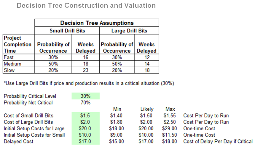
Figure 23.1: Decision tree assumptions
Using these assumptions, a simple decision tree can be constructed. The decision tree is a graphical representation of decisions, probabilities of outcomes, and payoffs given certain outcomes, based on a chronological order. The value of each branch on the tree is then computed using backward induction or expected value analysis. The decision tree is constructed as seen in Figure 23.2.
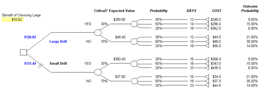
Figure 23.2: Decision tree construction
The payoffs at the terminal nodes of the decision tree are computed based on the path undertaken. For instance, $248M is computed by:
Initial Setup Cost of Large Drill Bit + Number of Days Delayed *
(Cost of Large Drill Bits Per Day + Delay Cost Per Day)
and so forth. Then, the expected values are computed using a backward induction. For instance, $289.80M is computed by:
30% ($248) + 50% ($286) + 20% ($362)
and the expected value at initiation for the Large Bit Drill of $120.82M is computed by:
30% ($289.80) + 70% ($48.40)
The benefit of choosing the large drill bit is the difference between the $120.82M and $131.44M costs, or $10.62M in cost savings. That is, the decision with the lowest cost is to go with the large drill bit. The computations of all remaining nodes on the tree are visible in the model.
Monte Carlo Simulation
The inputs above are single-point estimates and using them as-is will reduce the robustness of the model. By adding in input assumptions and probability distributions, the analysis can then be run through a Monte Carlo simulation in Risk Simulator. The highlighted values in Figures 23.1 and 23.2 are set up as simulation input assumptions and the resulting forecast output is the benefit of choosing the large drill bit. To run the simulation, simply:
- Click on Risk Simulator | Change Simulation Profile and select the Decision Tree Basics profile.
- Go to the Model worksheet and click on Risk Simulator | Run Simulation or click on the RUN icon.
The output forecast chart obtained after running the simulation is shown in Figure 23.3. Once the simulation is complete, go to the forecast chart and select Right Tail and type in 0 in the right-tail input box and hit TAB on the keyboard. The results show that there is a 97.50% probability that choosing Large Drill Bits will be worth more than Small Drill Bits (Figure 23.3), that is, the net benefit exceeds zero.
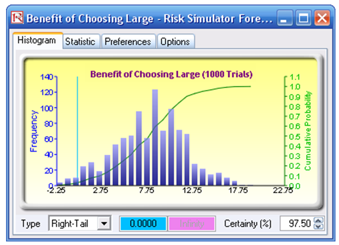
Figure 23.3: Simulating a decision tree
You are now ready to continue on to more sophisticated decision tree analyses. Please refer to the next chapter, Decision Tree with EVPI, Minimax and Bayes’ Theorem, for an example of more advanced decision tree analytics.
Pros and Cons of Decision Tree Analysis
As you can see, a decision tree analysis can be somewhat cumbersome, with all the associated decision analysis techniques. In creating a decision tree, be careful of its pros and cons. Specifically:
Pros
- Easy to use, construct, and value. Drawing the decision treemerely requires an understanding of the basics (e.g., the chronological sequence of events, payoffs, probabilities, decision nodes, chance nodes, and so forth; the valuation is simply expected values going from right to left on the decision tree).
- Clear and easy exposition. A decision tree is simple to visualize and understand.
Cons
- Ambiguous inputs. The analysis requires single-point estimates of many variables (many probabilities and many payoff values), and sometimes it is difficult to obtain objective or valid estimates. In a large decision tree, these errors in estimations compound over time, making the results highly ambiguous. The problem of garbage-in-garbage-out is clearly an issue here. Monte Carlo simulation with Risk Simulator helps by simulating the uncertain input assumptions thousands of times, rather than relying on single-point estimates.
- Ambiguous outputs. The decision tree results versus Minimax and Maximin results produce different optimal strategies as illustrated in the next chapter’s more complex decision tree example. Using decision trees will not necessarily produce robust and consistent results. Great care should be taken.
- Difficult and confusing mathematics. To make the decision tree analysis more powerful (rather than simply relying on single-point estimates), we revert to using Bayes’ Theorem. From the next chapter’s decision tree example, using the Bayes’ Theorem to derive implied and posterior probabilities is not an easy task at all. At best it is confusing and at worst, extremely complex to derive.
- In theory, each payoff value faces a different risk structure on the terminal nodes. Therefore, it is theoretically correct only if the payoff values (which have to be in present values) are discounted at different risk-adjusted discount rates, corresponding to the risk structure at the appropriate nodes. Obtaining a single valid discount rate is difficult enough, let alone multiple discount rates.
- The conditions, probabilities, and payoffs should be correlated to each other in real life. In a simple decision tree, this is not possible as you cannot correlate two or more probabilities. This is where Monte Carlo simulation comes in because it allows you to correlate pairs of input assumptions in a simulation.
- Decision trees do not solve real options! Be careful as real options analysis requires binomial and multinomial lattices and trees to solve, not decision tree Decision trees are great for framing strategic real options pathways but not for solving real options values. For instance, decision trees cannot be used to solve a switching option, or barrier option or option to expand, contract, and abandon. The branches on a decision tree are outcomes, while the branches on a lattice in a real option are options, not obligations. They are very different animals, so care should be taken when setting up real options problems versus decision tree problems. See Parts II and III of this book for more advanced cases involving real options problems and models.