File Names: Real Options – Abandonment American Option; Real Options – Abandonment Bermudan Option; Real Options – Abandonment Customized Option; Real Options – Abandonment European Option
Location: Modeling Toolkit | Real Options Models
Brief Description: Computes the abandonment option assuming American, Bermudan, and European flavors as well as customized inputs and parameters to mirror real-life situations using closed-form models and customized binomial lattices
Requirements: Modeling Toolkit, Real Options SLS
The Abandonment Option looks at the value of a project’s or asset’s flexibility in being abandoned over the life of the option. As an example, suppose that a firm owns a project or asset and that, based on traditional discounted cash flow (DCF) models, it estimates the present value of the asset (PV Underlying Asset) to be $120M. For the abandonment option, this is the net present value of the project or asset. Monte Carlo simulation using the Risk Simulator software indicates that the Volatility of this asset value is significant, estimated at 25%. Under these conditions, there is a lot of uncertainty as to the success or failure of this project. The volatility calculated models the different sources of uncertainty and computes the risks in the DCF model including price uncertainty, probability of success, competition, cannibalization, and so forth. Thus, the value of the project might be significantly higher or lower than the expected value of $120M. Suppose an abandonment option is created whereby a counterparty is found and a contract is signed that lasts five years (Maturity) such that for some monetary consideration now, the firm has the ability to sell the asset or project to the counterparty at any time within these five years (indicative of an American option) for a specified Salvage of $90M. The counterparty agrees to this $30M discount and signs the contract.
What has just occurred is that the firm bought itself a $90M insurance policy. That is, if the asset or project value increases above its current value, the firm may decide to continue funding the project, or sell it off in the market at the prevailing fair market value. Alternatively, if the value of the asset or project falls below the $90M threshold, the firm has the right to execute the option and sell off the asset to the counterparty at $90M. In other words, a safety net of sorts has been erected to prevent the value of the asset from falling below this salvage level. Thus, how much is this safety net or insurance policy worth? You can create a competitive advantage in negotiation if the counterparty does not have the answer and you do. Further, assume that the five-year Treasury Note Risk-Free Rate (zero coupon) is 5% from the U.S. Department of Treasury (http://www.treasury.gov). The American Abandonment Option results in Figure 180.1 show a value of $125.48M, indicating that the option value is $5.48M as the present value of the asset is $120M. Hence, the maximum value you should be willing to pay for the contract on average is $5.48M. This resulting expected value weights the continuous probabilities that the asset value exceeds $90M versus when it does not (where the abandonment option is valuable). Also, it weights when the timing of executing the abandonment is optimal such that the expected value is $5.48M.
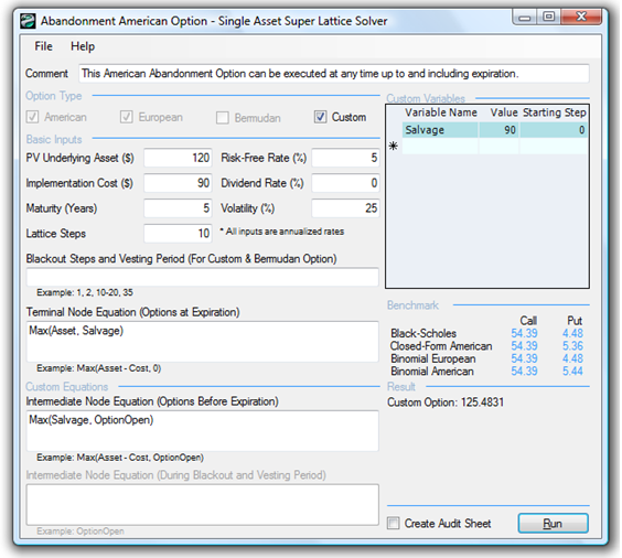
Figure 180.1: Simple American abandonment option
In addition, some experimentation can be conducted. Changing the salvage value to $30M (this means a $90M discount from the starting asset value) yields a result of $120M, or $0M for the option. This result means that the option or contract is worthless because the safety net is set so low that it will never be utilized. Conversely, setting the salvage level to three times the prevailing asset value, or $360M, would yield a result of $360M, and the options valuation results indicate $360M, which means that there is no option value; there is no value in waiting and having this option, or simply, execute the option immediately and sell the asset if someone is willing to pay three times the value of the project right now. Thus, you can keep changing the salvage value until the option value disappears, indicating the optimal trigger value has been reached. For instance, if you enter $166.80 as the salvage value, the abandonment option analysis yields a result of $166.80, indicating that at this price and above, the optimal decision is to sell the asset immediately, given the assumed volatility and the other input parameters. At any lower salvage value, there is option value, and at any higher salvage value, there will be no option value. This break-even salvage point is the optimal trigger value. Once the market price of this asset exceeds this value, it is optimal to abandon. Finally, adding a Dividend Rate, the cost of waiting before abandoning the asset (e.g., the annualized taxes and maintenance fees that have to be paid if you keep the asset and not sell it off, measured as a percentage of the present value of the asset) will decrease the option value. Hence, the break-even trigger point, where the option becomes worthless, can be calculated by successively choosing higher dividend levels. This break-even point again illustrates the trigger value at which the option should be optimally executed immediately, but this time with respect to a dividend yield. That is, if the cost of carry or holding on to the option, or the option’s leakage value is high (i.e., if the cost of waiting is too high), do not wait and execute the option immediately.
Other applications of the abandonment option include buy-back lease provisions in a contract (guaranteeing a specified asset value); asset preservation flexibility; insurance policies; walking away from a project and selling off its intellectual property; purchase price of an acquisition; and so forth. To illustrate, here are some additional examples of the abandonment option:
- An aircraft manufacturer sells its planes of a particular model in the primary market for, say, $30M each to various airline companies. Airlines are usually risk-averse and may find it hard to justify buying an additional plane with all the uncertainties in the economy, demand, price competition, and fuel costs. When uncertainties become resolved over time, actions, and events, airline carriers may have to reallocate and reroute their existing portfolio of planes globally, and an excess plane on the tarmac is very costly. The airline can sell the excess plane in the secondary market where smaller regional carriers buy used planes, but the price uncertainty is very high and is subject to significant volatility, of, say, 45%, and may fluctuate wildly between $10M and $25M for this class of aircraft. The aircraft manufacturer can reduce the airline’s risk by providing a buyback provision or abandonment option, where at any time within the next five years, the manufacturer agrees to buy back the plane at a guaranteed residual salvage price of $20M, at the request of the airline. The corresponding risk-free rate for the next five years is 5%. This reduces the downside risk of the airline, and hence reduces its risk, chopping off the left tail of the price fluctuation distribution, and shifting the expected value to the right. This abandonment option provides risk reduction and value enhancement to the airline. Applying the abandonment option in SLS using a 100-step binomial lattice, we find that this option is worth $3.52M. If the airline is the smarter counterparty and calculates this value and gets this buyback provision for free as part of the deal, the aircraft manufacturer has just left over 10% of its aircraft value on the negotiation table. Information and knowledge is highly valuable in this case.
- A high-tech disk-drive manufacturer is thinking of acquiring a small start-up firm with a new microdrive technology (a super-fast and high-capacity pocket hard drive) that may revolutionize the industry. The start-up is for sale and its asking price is $50M based on an NPV fair market value analysis some third-party valuation consultants have performed. The manufacturer can either develop the technology itself or acquire this technology through the purchase of the firm. The question is, how much is this firm worth to the manufacturer, and is $50M a good price? Based on internal analysis by the manufacturer, the NPV of this microdrive is expected to be $45M, with a cash flow volatility of 40%, and it would take another three years before the microdrive technology is successful and goes to market. Assume that the three-year risk-free rate is 5%. In addition, it would cost the manufacturer $45M in present value to develop this drive internally. If using an NPV analysis, the manufacturer should build the drive itself. However, if you include an abandonment option analysis whereby if this specific microdrive does not work, the start-up still has an abundance of intellectual property (patents and proprietary technologies) as well as physical assets (buildings and manufacturing facilities) that can be sold in the market at up to $40M, the abandonment option together with the NPV yields $51.83, making buying the start-up worth more than developing the technology internally, and making the purchase price of $50M worth it. (See the section on Expansion Option for more examples on how this start-up’s technology can be used as a platform to further develop newer technologies that can be worth a lot more than just the abandonment option.)
Real Options – Abandonment American Option
Figure 180.1 shows the results of a simple abandonment option with a 10-step lattice as discussed, while Figure 180.2 shows the audit sheet that is generated from this analysis.
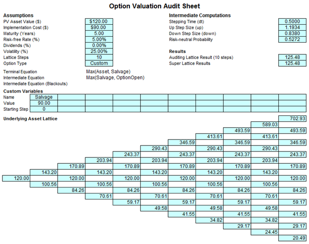
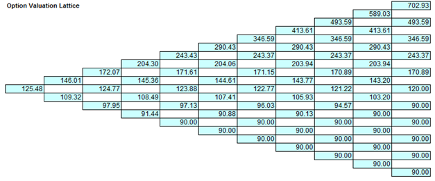
Figure 180.2 Audit sheet for the abandonment option
Figure 180.3 shows the same abandonment option but with a 100-step lattice. To follow along, open the example file by first starting the SLS software. Then click on Single Asset Option Model and then File | Examples | Abandonment American Option. Notice that the 10-step lattice yields $125.48 while the 100-step lattice yields $125.45, indicating that the lattice results have achieved convergence. The Terminal Node Equation is Max(Asset, Salvage), which means the decision at maturity is to decide if the option should be executed, selling the asset and receiving the salvage value, or not to execute, holding on to the asset. The Intermediate Node Equation used is Max(Salvage, OptionOpen) indicating that before maturity, the decision is either to execute early in this American option to abandon and receive the salvage value, or to hold on to the asset and, hence, hold on to and keep the option open for potential future execution, denoted simply as OptionOpen.
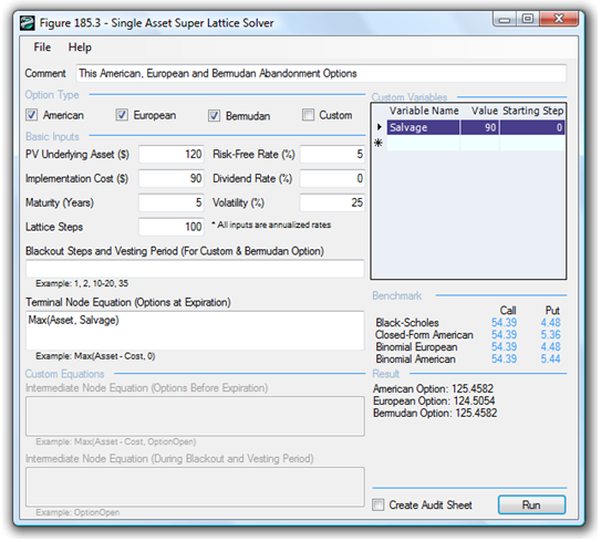
Figure 180.3: American, European, and Bermudan Abandonment option with 100-step lattice
Real Options – Abandonment European Option
Figure 180.4 shows the European version of the abandonment option, where the Intermediate Node Equation is simply Option Open, as early execution is prohibited before maturity. Of course, being able to execute the option only at maturity is worth less ($124.5054 compared to $125.4582) than being able to exercise earlier. The example files used are Abandonment American Option and Abandonment European Option. For example, the airline manufacturer in the previous case example can agree to a buy-back provision that can be exercised at any time by the airline customer versus only at a specific date at the end of five years––the former American option will clearly be worth more than the latter European option.
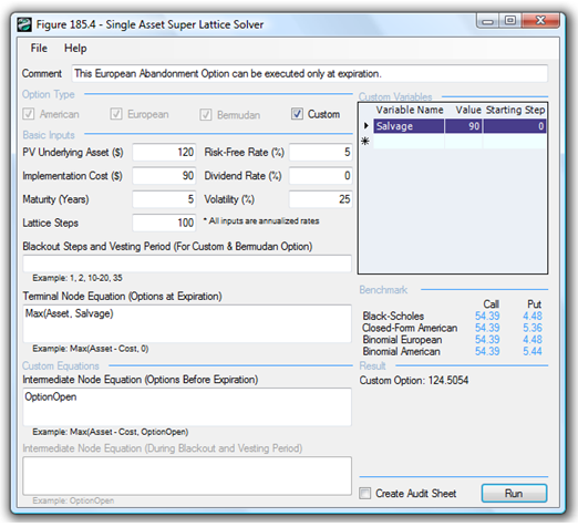
Figure 180.4: European abandonment option with 100-step lattice
Real Options – Abandonment Bermudan Option
Sometimes, a Bermudan option is appropriate, as when there might be a vesting period or blackout period when the option cannot be executed. For instance, if the contract stipulates that for the 5-year abandonment buyback contract, the airline customer cannot execute the abandonment option within the first 2.5 years. This is shown in Figure 180.5 using a Bermudan option with a 100-step lattice on 5 years, where the blackout steps are from 0-50. This means that during the first 50 steps (as well as right now or step 0), the option cannot be executed. This is modeled by inserting Option Open into the Intermediate Node Equation During Blackout and Vesting Periods. This forces the option holder only to keep the option open during the vesting period, preventing execution during this blackout period.
Figure 180.5 shows that the American option is worth more than the Bermudan option, which is worth more than the European option, by virtue of the ability of each option type to execute early and the frequency of execution possibilities.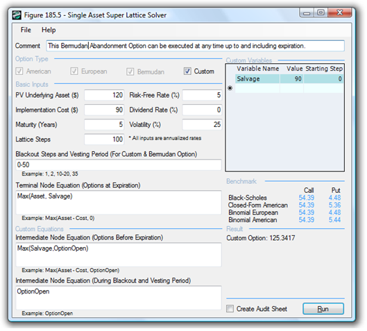
Figure 180.5: Bermudan abandonment option with 100-step lattice
Real Options – Abandonment Customized Option
Sometimes, the salvage value of the abandonment option may change over time. To illustrate, in the previous example of an acquisition of a start-up firm, the intellectual property will most probably increase over time because of continued research and development activities, thereby changing the salvage values over time. An example is seen in Figure 180.6, where there are five salvage values over the five-year abandonment option. This can be modeled by using the Custom Variables. Type in the input variables one at a time as seen in Figure 180.6’s Custom Variables list. Notice that the same variable name (Salvage) is used but the values change over time, and the starting steps represent when these different values become effective. For instance, the salvage value of $90 applies at step 0 until the next salvage value of $95 takes over at step 21. This means that for a five-year option with a 100-step lattice, the first year including the current period (steps 0 to 20) will have a salvage value of $90, which then increases to $95 in the second year (steps 21 to 40), and so forth. Notice that as the value of the firm’s intellectual property increases over time, the option valuation results also increase, which makes logical sense. You can also model in blackout vesting periods for the first six months (steps 0-10 in the blackout area). The blackout period is very typical of contractual obligations of abandonment options where during specified periods, the option cannot be executed (a cooling-off period).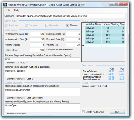
Figure 180.6: Customized abandonment option
Exercise: Option to Abandon
Suppose a pharmaceutical company is developing a particular drug. However, due to the uncertain nature of the drug’s development progress, market demand, success in human and animal testing, and Food and Drug Administration approval, management has decided that it will create a strategic abandonment option. That is, at any time period within the next five years of development, management can review the progress of the research and development effort and decide whether to terminate the drug development program. After five years, the firm would have either succeeded or completely failed in its drug development initiative, and there exists no option value after that time period. If the program is terminated, the firm can potentially sell off its intellectual property rights to the drug in question to another pharmaceutical firm with which it has a contractual agreement. This contract with the other firm is exercisable at any time within this time period, at the whim of the firm owning the patents.
Using a traditional DCF model, you find the present value of the expected future cash flows discounted at an appropriate market risk-adjusted discount rate to be $150 million. Using Monte Carlo simulation, you find the implied volatility of the logarithmic returns on future cash flows to be 30%. The risk-free rate on a riskless asset for the same time frame is 5%, and you understand from the intellectual property officer of the firm that the value of the drug’s patent is $100 million contractually, if sold within the next five years. For simplicity, you assume that this $100 million salvage value is fixed for the next five years. You attempt to calculate how much this abandonment option is worth and how much this drug development effort, on the whole, is worth to the firm. By virtue of having this safety net of being able to abandon drug development, the value of the project is worth more than its net present value. You decide to use a closed-form approximation of an American put option because the option to abandon drug development can be exercised at any time up to and including the expiration date. You also decide to confirm the value of the closed-form analysis with a binomial lattice calculation. With these assumptions, do the following exercises, answering the questions posed:
- Solve the abandonment option problem manually using a 10-step lattice and confirm the results by generating an audit sheet using the SLS software.
- Select the right choice for each of the following:
- Increases in maturity (increase/decrease) an abandonment option value.
- Increases in volatility (increase/decrease) an abandonment option value.
- Increases in asset value (increase/decrease) an abandonment option value.
- Increases in risk-free rate (increase/decrease) an abandonment option value.
- Increases in dividend (increase/decrease) an abandonment option value.
- Increases in salvage value (increase/decrease) an abandonment option value.
- Apply 100 steps using the software’s binomiallattice.
- How different are the results as compared to the 5-step lattice?
- How close are the closed-form results compared to the 100-step lattice?
- Apply a 3% continuous dividend yield to the 100-step lattice.
- What happens to the results?
- Does a dividend yield increase or decrease the value of an abandonment option? Why?
- Assume that the salvage value increases at a 10% annual rate. Show how this can be modeled using the software’s Custom Variables List.
- Explain the differences in results when using the Black-Scholes and American Put Option Approximation in the benchmark section of the Single Asset SLS software.