File Name: Project Management – Critical Path Analysis (CPM PERT GANTT)
Location: Modeling Toolkit | Project Management | Critical Path Analysis (CPM PERT GANTT)
Brief Description: Illustrates how to use Risk Simulator for running simulations on time to completion of a project and critical path determination, creating GANTT charts and CPM/PERT models, simulating dates and binary variables, and linking input assumptions
Requirements: Modeling Toolkit, Risk Simulator
This model illustrates how a Project Management Critical Path Analysis and completion times can be modeled using Risk Simulator. The typical inputs of minimum, most likely, and maximum duration of each process or subproject can be modeled using the triangular distribution. This distribution typically is used in the Critical Path Method (CPM) and Program Evaluation Review Technique (PERT) in project management, together with the beta distribution. In other words, the assumptions in the model can also take the beta and gamma distributions rather than the triangular distribution. However, the beta and gamma distributions are more complex for project managers to use, hence the popularity of the triangular distribution.
In this two-part model, the first is a CPM critical path analysis to determine the critical path as well as the expected completion time of a project (Figure 118.1). The second part of the model is on the same project, but we are interested in the actual potential completion date with a GANTT chart analysis (Figure 118.2).
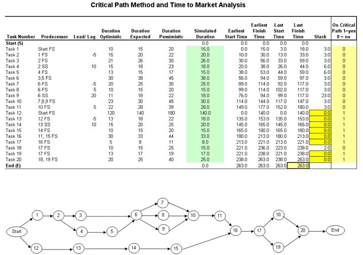
Figure 118.1: Critical path model and time to market analysis
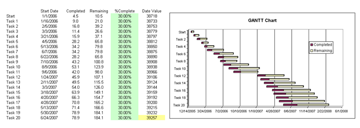
Figure 118.2: GANTT chart
Procedure
- The cells in column G in the model already have simulation assumptions To view the assumptions, select cell G5 and click on Risk Simulator | Set Input Assumption. You will see that a triangular distribution is set where the input parameters (minimum, most likely, and maximum) are linked to the corresponding cells in columns D to F (Figure 118.3). Note that when you click on the input parameters, you will see the links to D5, E5, and F5. Notice also that the input parameter boxes are now colored light green, indicating that the parameters are linked to a cell in the spreadsheet. If you entered or hard-coded a parameter, it would be white. You can link a parameter input to a cell in a worksheet by clicking on the link icon (beside the parameter input box) and clicking on the relevant cell in the worksheet.
- For simplicity, other assumption shave already been preset for you, including the completion percentage in Column E of the second part of the model, where we use the beta distribution Further, several forecasts have been set, including the Finish Time (L25), Ending Date (F63), and critical path binary values (N5:N24) for various tasks. All that needs to be done now is to run the simulation: Risk Simulator | Run Simulation.
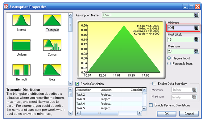
Figure 118.3: Setting the input assumptions
Results Interpretation
Several results are noteworthy:
- Looking at the Finish Time forecast chart after the simulation is completed, select Left-Tail and enter 95 in the Certainty box, and hit TAB on the keyboard (Figure 118.4). This shows a value of 301.71, which means that there is a 95% chance that the project will complete in slightly under 302 days or that only a 5% chance exists where there will be an overrun of 301 days. Similarly, you can enter in 285 in the Value box and hit TAB. The forecast chart returns a value of 69.60%, indicating that there is only a 69.60% chance that the project can finish within 285 days, or a 30.40% chance the project will take longer than 285 days. Other values can be entered similarly.
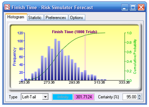

Figure 118.4: Forecast results
- Select one of the Tasks (e.g., Task 10). The forecast chart is bimodal, with two peaks, one at 0 and another at 1, indicating “NO” and “YES” on whether this particular task ends up being on the critical path (Figure 118.5). In this example, select the Left-Tail and type in 99, and hit TAB on the keyboard. Notice that the certainty value is 58.20%, indicating that this project has a 58.20% chance of not being on the critical path (the value 0) or a 41.80% chance of being on the critical path (the value 1). This means that Task 10 is potentially very critical. In contrast, look at Task 9’s forecast chart. The Left-Tail certainty is 100% at the value of 0.99, indicating that 100% of the time, this project is not going to be on the critical path, and therefore has less worry for the project manager.
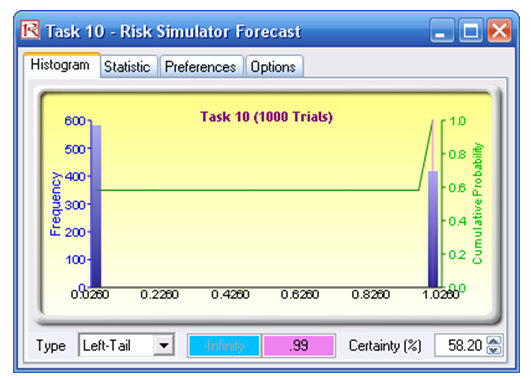
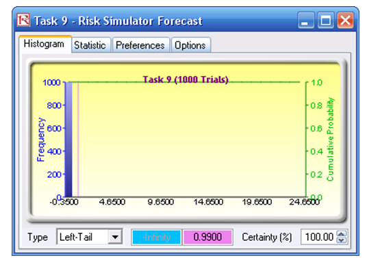
Figure 118.5: Task forecast
- Finally, the Ending Date forecast can be used to determine the potential ending date of the project. Looking at the forecast chart output, select the Left-Tail, enter 95, and hit TAB (Figure 118.6). The corresponding 95th percentile returns a value of 39301. This is a text format for a specific date in Excel. To convert it into a date we understand, simply type this number in any empty cell and click on Format | Cells (or hit Ctrl-1) and select Number | Date, and the cell value changes to August 7, 2007. This means that there is a 95% chance that the project will be completed by August 7, 2007.
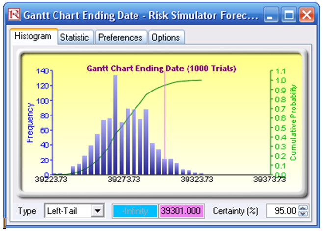
Figure 118.6: GANTT chart forecast end date
You can now experiment with other values and certainty levels as well as modify the model to suit your needs and project specifications. In addition, you can use the same methodology to simulate binary values (variables with 0/1 values) and dates.