RUNNING A MONTE CARLO SIMULATION

Typically, to run a simulation in your existing Excel model, the following steps have to be performed:

1. Start a new simulation profile or open an existing profile.
2. Define input assumptions in the relevant cells.
3. Define output forecasts in the relevant cells.
4. Run simulation.
5. Interpret the results.

If desired, and for practice, open the example file called Basic Simulation Model and follow along with the examples provided here on creating a simulation. The example file can be found by first starting Excel, and then clicking on Risk Simulator | Example Models | 02 Basic Simulation Model.

 1.  Start a New Simulation Profile

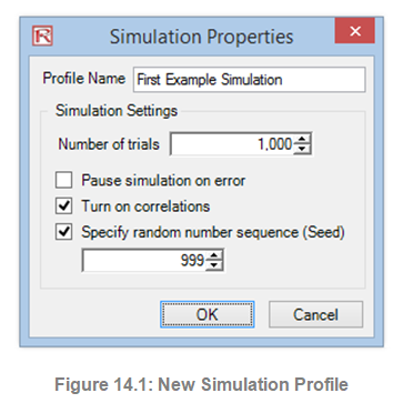
To start a new simulation, you must first create a simulation profile (Figure 14.1). A simulation profile contains a complete set of instructions on how you would like to run a simulation (i.e., all the assumptions, forecasts, run preferences, and so forth). Having profiles facilitates creating multiple scenarios of simulations. That is, using the same exact model, several profiles can be created, each with its own specific simulation properties and requirements. The same person can create different test scenarios using different distributional assumptions and inputs, or multiple persons can test their own assumptions and inputs on the same model.

• Start Excel and create a new or open an existing model (you can use the Basic Simulation Model example to follow along).
• Click on Risk Simulator | New Simulation Profile.
• Specify a title for your simulation as well as all other pertinent information.

The following explains the user input requirements in Figure 14.1:

• Title. Specifying a simulation title allows you to create multiple simulation profiles in a single Excel model. Using a title means that you can now save different simulation scenario profiles within the same model without having to delete existing assumptions and changing them each time a new simulation scenario is required. You can always change the profile’s name later (Risk Simulator | Edit Profile).
• Number of Trials. This is where the number of simulation trials required is entered. That is, running 1,000 trials means that 1,000 different iterations of outcomes based on the input assumptions will be generated. You can change this as desired, but the input has to be positive integers. The default number of runs is 1,000 trials. You can use precision and error control to automatically help determine how many simulation trials to run (see the section on precision and error control later in this chapter for details).
• Pause Simulation on Error. If checked, the simulation stops every time an error is encountered in the Excel model. That is, if your model encounters a computation error (e.g., some input values generated in a simulation trial may yield a divide by zero error in one of your spreadsheet cells), the simulation stops. This feature is important to help audit your model to make sure there are no computational errors in your Excel model. However, if you are sure the model works, then there is no need for this preference to be checked.
• Turn On Correlations. If checked, correlations between paired input assumptions will be computed. Otherwise, correlations will all be set to zero, and a simulation is run assuming no cross-correlations between input assumptions. As an example, applying correlations will yield more accurate results if indeed correlations exist and will tend to yield a lower forecast confidence if negative correlations exist. After turning on correlations here, you can later set the relevant correlation coefficients on each assumption generated (see the section on correlations and precision control later in this chapter for more details).
• Specify Random Number Sequence. Simulation, by definition, will yield slightly different results every time a simulation is run. Different results occur by virtue of the random number generation routine in Monte Carlo simulation; this characteristic is a theoretical fact in all random number generators. However, when making presentations, if you require the same results (especially if you have already run a simulation and generated a report to present a set of results, and you would like to show the same results being generated in a live presentation; or when you are sharing models with others and would like the same results to be obtained every time), then check this preference and enter in an initial seed number. The seed number can be any positive integer. Using the same initial seed value, the same number of trials, and the same input assumptions, the simulation will always yield the same sequence of random numbers, guaranteeing the same final set of results.

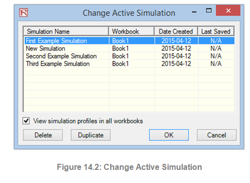
Note that once a new simulation profile has been created, you can come back later and modify these selections. In order to do this, make sure that the current active profile is the profile you wish to modify, otherwise, click on Risk Simulator | Change Simulation Profile, select the profile you wish to change, and click OK (Figure 14.2 shows an example where there are multiple profiles and how to activate a selected profile). Then, click on Risk Simulator | Edit Simulation Profile and make the required changes. You can also duplicate or rename an existing profile. When creating multiple profiles in the same Excel model, make sure to provide each profile a unique name so you can tell them apart later on. Also, these profiles are stored inside hidden sectors of the Excel *.xlsx file and you do not have to save any additional files. The profiles and their contents (assumptions, forecasts, etc.) are automatically saved when you save the Excel file. Finally, the last profile that is active when you exit and save the Excel file will be the one that is opened the next time the Excel file is accessed.

2.  Define Input Assumptions

The next step is to set input assumptions in your model. Note that assumptions can only be assigned to cells without any equations or functions (i.e., typed-in numerical values that are inputs in a model), whereas output forecasts can only be assigned to cells with equations and functions (i.e., outputs of a model). Recall that assumptions and forecasts cannot be set unless a simulation profile already exists. Do the following to set new input assumptions in your model:

1. Make sure a Simulation Profile exists, open an existing profile, or start a new profile (Risk Simulator | New Simulation Profile).
2. Select the cell you wish to set an assumption on (e.g., cell G8 in the Basic Simulation Model example).
3. Click on Risk Simulator | Set Input Assumption or click on the set input assumption icon in the Risk Simulator icon toolbar.
4. Select the relevant distribution you want, enter the relevant distribution parameters (e.g., select Triangular distribution and use 1, 2, and 2.5 as the minimum, most likely, and maximum values), and hit OK to insert the input assumption into your model (Figure 14.3).

Note that you can also set assumptions by selecting the cell you wish to set the assumption on and, using the mouse right-click, access the shortcut Risk Simulator menu to set an input assumption.

In addition, for expert users, you can set input assumptions using the Risk Simulator RS Functions: select the cell of choice, click on Excel’s Insert, Function, and select the All Category, and scroll down to the RS functions list (we do not recommend using RS functions unless you are an expert user). For the examples going forward, we suggest following the basic instructions in accessing menus and icons.

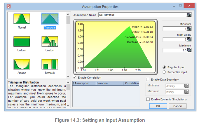
Notice that in the Assumption Properties, there are several key areas worthy of mention. Figure 14.4 shows the different areas:

• Assumption Name. This is an optional area that allows you to enter in unique names for the assumptions to help track what each of the assumptions represents. Good modeling practice is to use short but precise assumption names.
• Distribution Gallery. This area to the left shows the 50 different probability distributions available in the software. To change the views, right-click anywhere in the gallery and select large icons, small icons, or lists.
• Input Parameters. Depending on the distribution selected, the required relevant parameters are shown. You may either enter the parameters directly or link them to specific cells in your worksheet. Hard coding or typing the parameters is useful when the assumption parameters are assumed not to change. Linking to worksheet cells is useful when the input parameters need to be visible or are allowed to be changed (click on the link icon to link an input parameter to a worksheet cell).
• Enable Data Boundary. This feature is typically not used by the average analyst but exists for truncating the distributional assumptions. For instance, if a normal distribution is selected, the theoretical boundaries are between negative infinity and positive infinity. However, in practice, the simulated variable exists only within some smaller range, and this range can then be entered to truncate the distribution appropriately.
• Pairwise correlations can be assigned to input assumptions here. If correlations are required in the simulation model, remember to check the Turn on Correlations preference by clicking on Risk Simulator |Edit Simulation Profile. See the discussion on correlations later in this chapter for more details about assigning correlations and the effects correlations have on a model. Notice that you can either truncate a distribution or correlate it to another assumption but not both.
• Short Descriptions. These exist for each of the distributions in the gallery. The short descriptions explain when a certain distribution is used as well as the input parameter requirements.
• Regular Input and Percentile Input. This option allows the user to perform a quick due diligence test of the input assumption. For instance, if setting a normal distribution with some mean and standard deviation inputs, you can click on the percentile input to see what the corresponding 10th and 90th percentiles are.
• Enable Dynamic Simulations. This option is unchecked by default, but if you wish to run a multidimensional simulation (i.e., if you link the input parameters of the assumption to another cell that is itself an assumption, you are simulating the inputs, or simulating the simulation), then remember to check this option. Dynamic simulation will not work unless the inputs are linked to other changing input assumptions.

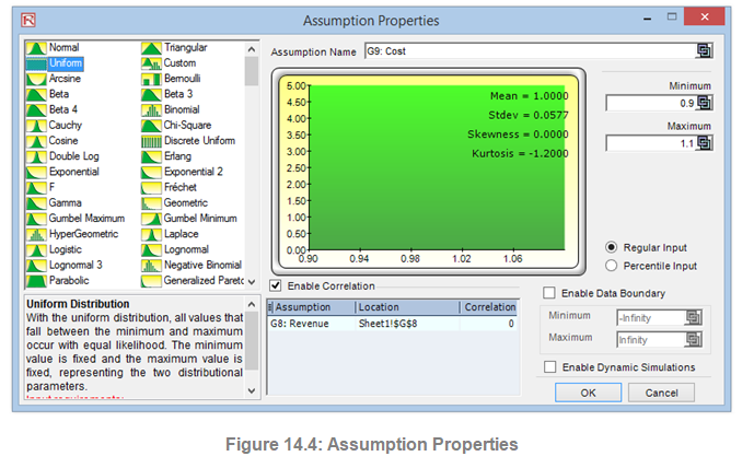
Note: If you are following along with the example, continue by setting another assumption on cell G9. This time use the Uniform distribution with a minimum value of 0.9 and a maximum value of 1.1. Then, proceed to define the output forecasts in the next step.

 3. Define Output Forecasts

The next step is to define output forecasts in the model. Forecasts can only be defined on output cells with equations or functions. The following describes the set forecast process:

1. Select the cell you wish to set an assumption on (e.g., cell G10 in the Basic Simulation Model example).
2. Click on Risk Simulator | Set Output Forecast or click on the set output forecast icon on the Risk Simulator icon toolbar.
3. Enter the relevant information and click OK.

Note that you can also set output forecasts by selecting the cell you wish to set the assumption on and, using the mouse right-click, access the shortcut Risk Simulator menu to set an output forecast.

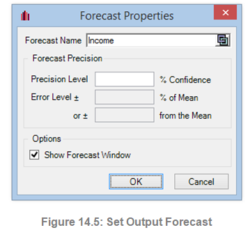
Figure 14.5 illustrates the set forecast properties:

• Forecast Name. Specify the name of the forecast This is important because when you have a large model with multiple forecast cells, naming the forecast cells individually allows you to access the right results quickly. Do not underestimate the importance of this simple step. Good modeling practice is to use short but precise assumption names.
• Forecast Precision. Instead of relying on a guesstimate of how many trials to run in your simulation, you can set up precision and error control When an error-precision combination has been achieved in the simulation, the simulation will pause and inform you of the precision achieved, making the number of simulation trials an automated process and eliminating guesses on the required number of trials to simulate. Review the section on precision and error control later in this chapter for more specific details.
• Show Forecast Window. This property allows the user to show or not show a particular forecast  The default is to always show a forecast chart.

4. Run Simulation

If everything looks right, simply click on Risk Simulator | Run Simulation or click on the Run icon on the Risk Simulator toolbar and the simulation will proceed. You may also reset a simulation after it has run to rerun it (Risk Simulator | Reset Simulation or the reset simulation icon on the toolbar) or to pause it during a run. Also, the step function (Risk Simulator | Step Simulation or the step simulation icon on the toolbar) allows you to simulate a single trial, one at a time, useful for educating others on simulation (i.e., you can show that at each trial, all the values in the assumption cells are being replaced and the entire model is recalculated each time). You can also access the run simulation menu by right-clicking anywhere in the model and selecting Run Simulation.

Risk Simulator also allows you to run the simulation at an extremely fast speed, called Super Speed. To do this, click on Risk Simulator | Run Super Speed Simulation or use the run super speed icon. Notice how much faster the super speed simulation runs. In fact, for practice, click on Reset Simulation and then Edit Simulation Profile, change the Number of Trials to 100,000, and click on Run Super Speed. It should only take a few seconds to run. However, be aware that super speed simulation will not run if the model has errors, VBA (Visual Basic for Applications), or links to external data sources or applications. In such situations, you will be notified, and the regular speed simulation will be run instead. Regular speed simulations are always able to run even with errors, VBA, or external links.

 5. Interpret the Forecast Results

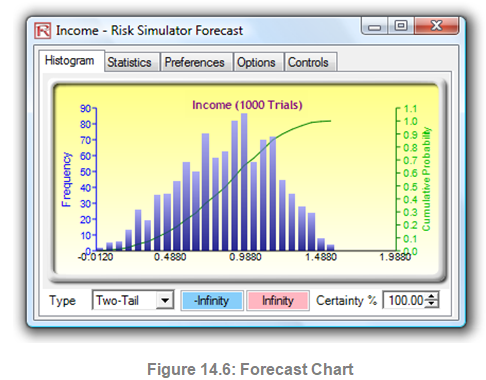
The final step in Monte Carlo simulation is to interpret the resulting forecast charts. Figures 14.6 through 14.13 show the forecast chart and the corresponding statistics generated after running the simulation. Typically, the following features are important in interpreting the results of a simulation:

• Forecast Chart. The forecast chart shown in Figure 14.6 is a probability histogram that shows the frequency counts of values occurring in the total number of trials  The vertical bars show the frequency of a particular x value occurring out of the total number of trials, while the cumulative frequency (smooth line) shows the total probabilities of all values at and below x occurring in the forecast.
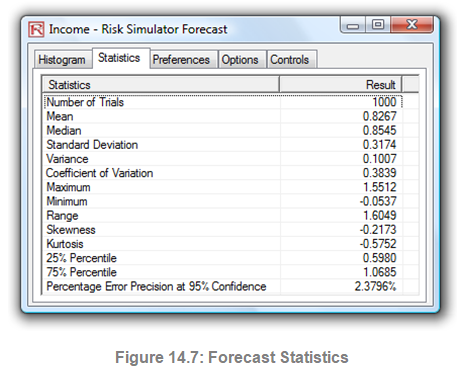
• Forecast Statistics. The forecast statistics shown in Figure 14.7 summarize the distribution of the forecast values in terms of the four moments of a distribution. See the section on understanding the forecast statistics in the previous chapter for more details on what some of these statistics mean. You can rotate between the histogram and statistics tab by depressing the space bar.

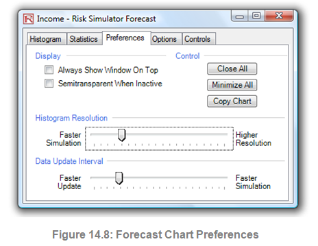
• Preferences. The preferences tab in the forecast chart (Figure 14.8) allows you to change the look and feel of the charts. For instance, if Always Show Window on Top is selected, the forecast charts will always be visible regardless of what other software applications are running on your computer. Histogram Resolution allows you to change the number of bins of the histogram, anywhere from 5 bins to 100 bins. Also, the Data Update Interval section allows you to control how fast the simulation runs versus how often the forecast chart is updated. That is, if you wish to see the forecast chart updated at almost every trial, this feature will slow down the simulation as more memory is being allocated to updating the chart versus running the simulation. This option is merely a user preference and in no way changes the results of the simulation, just the speed of completing the simulation. To further increase the speed of the simulation, you can minimize Excel while the simulation is running, thereby reducing the memory required to visibly update the Excel spreadsheet and freeing up the memory to run the simulation. The Close All and Minimize All controls both the open forecast charts, and Copy Chart allows you to copy the histogram into the clipboard where you can paste it into other applications.

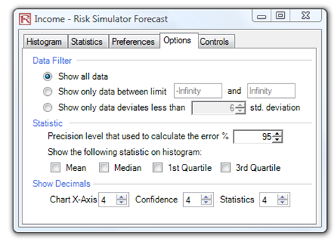
• Options. This forecast chart option (Figure 14.9, top) allows you to show all the forecast data or to filter in/out values that fall within some specified interval you choose, or within some standard deviation you choose. Also, the precision level can be set here for this specific forecast to show the error levels in the statistics  See the section on precision and error control later in this chapter for more details. Show the Following Statistic on Histogram is a user preference if the mean, median, first quartile, and fourth quartile lines (25th and 75th percentiles) should be displayed on the forecast chart. Preferences on the number of decimals to show in the chart, confidence intervals, and simulation statistics, can also be set here.
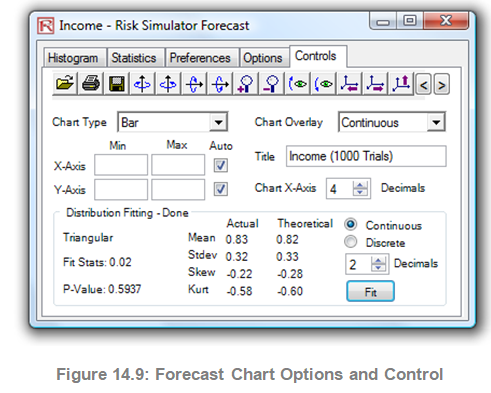
• Controls. This tab (Figure 14.9, bottom) has all the functionalities in allowing you to change the type, color, size, zoom, tilt, 3D, and other things in the forecast chart, as well as providing overlay charts (PDF, CDF) and running distributional fitting on your forecast data (see the Data Fitting sections in the previous chapter for more details on this methodology).