Basic simulations can be performed using Excel. However, more advanced simulation packages such as Risk Simulator perform the task more efficiently, in addition to having additional features preset in each simulation. We now present both Monte Carlo parametric simulation and nonparametric bootstrap simulation using Excel and Risk Simulator.
The examples in Figures 13.5 and 13.6 are created using Excel to perform a limited number of simulations on a set of probabilistic assumptions. We assume that having performed a series of scenario analyses, we obtain a set of nine resulting values, complete with their respective probabilities of occurrence. The first step in setting up a simulation in Excel for such a scenario analysis is to understand the function “RAND( )” within Excel. This function is simply a random number generator Excel uses to create random numbers from a uniform distribution between 0 and 1. Then it translates this 0 to 1 range using the assigned probabilities in our assumption into ranges or bins. For instance, if the value $362,995 occurs with a 55% probability, we can create a bin with a range of 0.00 to 0.55. Similarly, we can create a bin range of 0.56 to 0.65 for the next value of $363,522 which occurs 10% of the time, and so forth. Based on these ranges and bins, the nonparametric simulation can now be set up.
Figure 13.5 illustrates an example with 5,000 sets of trials. Each set of trials is simulated 100 times; that is, in each simulation trial set, the original numbers are picked randomly with replacement by using the Excel formula “VLOOKUP(RAND( ), $D$16:$F$24, 3)” which picks up the third column of data from the D16 to F24 area by matching the results from the RAND( ) function and data from the first column.
The average of the data sampled is then calculated for each trial set. The distribution of these 5,000 trial sets’ averages is obtained and the frequency distribution is shown at the bottom of Figure 13.5. According to the Central Limit Theorem, the average of these sample averages will approach the real true mean of the population at the limit. In addition, the distribution will most likely approach normality when a sufficient set of trials is performed. Clearly running this nonparametric simulation manually in Excel is fairly tedious. An alternative is to use Risk Simulator’s custom distribution, which does the same thing but in an infinitely faster and more efficient fashion. The chapter on Pandora’s Toolbox illustrates some of these simulation tools in more detail.
Nonparametric simulation is a very powerful tool but it is only applicable if data are available. Clearly, the more data there is, the higher the level of precision and confidence in the simulation results. However, when no data exist or when a valid systematic process underlies the dataset (e.g., physics, engineering, economic relationship, and so forth) parametric simulation may be more appropriate, where exact probabilistic distributions are used.
Using Excel to perform simulations is easy and effective for simple problems. However, when more complicated problems or requirements arise (e.g., correlations exist among input variables, dynamic sensitivities, reports and charts, simulation statistics, portfolio optimization, predictive modeling, stochastic processes, and many other such issues), the use of more specialized simulation packages are warranted. Risk Simulator is such a simulation package. In the example shown in Figure 13.7, the green-colored cells (Revenues, Opex, FCF/EBITDA) are the assumption cells, where we enter our distributional input assumptions, such as the type of distribution the variable follows and what the parameters are. For instance, we can say that revenues follow a normal distribution with a mean of $1,010 and a standard deviation of $100, based on analyzing historical revenue data for the firm. The net present value (NPV) cells are the forecast output cells, that is, the results of these cells are the results we ultimately wish to analyze. Refer to the next chapter, Test Driving Risk Simulator, for details on setting up and getting started with using the Risk Simulator software. The rest of this book is dedicated to modeling more complex requirements using the software.
Simulation(Probability Assumptions)
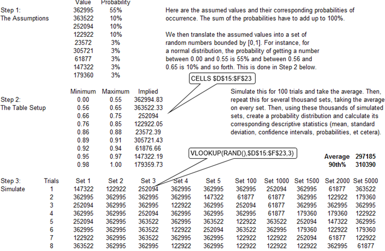
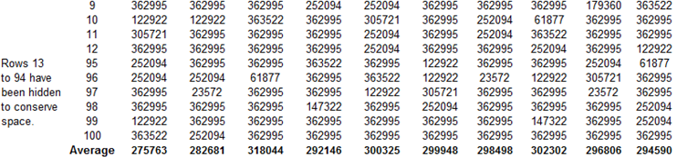
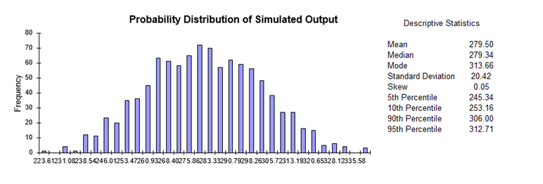
Figure 13.5: Simulation Using Excel I
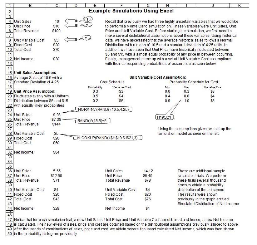
Figure 13.6: Simulation Using Excel II
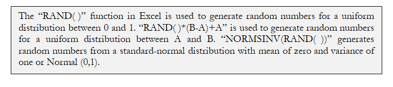
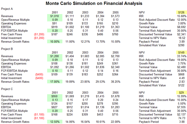
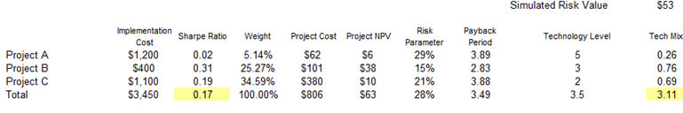
Figure 13.7: Simulation Using Risk Simulator