File Name: Probability of Default – Empirical
Location: Modeling Toolkit | Prob of Default | Empirical (Individuals)
Brief Description: Computes the probability of default on loans of individuals given some historical data on existing loans (age, educational levels, years at employment, etc.) and applies a maximum likelihood estimation approach
Requirements: Modeling Toolkit, Risk Simulator
The probability of default measures the degree of likelihood that the borrower of a loan or debt (also called an obligor) will be unable to make the necessary scheduled repayments on the debt, thereby defaulting on it. Should the obligor be unable to pay, the debt is in default, and the lenders of the debt have legal avenues to attempt a recovery of the debt, or at least partial repayment of the entire debt. The higher the default probability a lender estimates a borrower to have, the higher the interest rate the lender will charge the borrower as compensation for bearing the higher default risk.
The probability of default models are categorized as structural or empirical. Structural models are presented over the next few sections, which look at a borrower’s ability to pay based on market data such as equity prices, market and book values of assets and liabilities, as well as the volatility of these variables. Hence, they are used predominantly to estimate the probability of default of companies and countries. In contrast, empirical models or credit scoring models as presented here are used to quantitatively determine the probability that a loan or loan holder will default, where the loan holder is an individual, by looking at historical portfolios of loans held, where individual characteristics are assessed (e.g., age, educational level, debt to income ratio, and so forth). Other default models in the Modeling Toolkit handle corporations using market comparables and asset/liability valuations as seen in the next section.
The data here represent a sample of several hundred previous loans, credit, or debt issues. The data show whether each loan had defaulted or not, as well as the specifics of each loan applicant’s age, education level (1–3 indicating high school, university, or graduate professional education), years with current employer, and so forth (Figure 3.2). The idea is to model these empirical data to see which variables affect the default behavior of individuals, using Risk Simulator’s Maximum Likelihood models. The resulting model will help the bank or credit issuer compute the expected probability of default of an individual credit holder having specific characteristics.
To run the analysis, select the data (include the headers) and make sure that the data have the same length for all variables, without any missing or invalid data. Then, click on Risk Simulator | Forecasting | Maximum Likelihood Models. A sample set of results is provided in the MLE worksheet in the model, complete with detailed instructions on how to compute the expected probability of default of an individual.
Maximum Likelihood Estimates (MLE) on a binary multivariate logistic analysis is used to model dependent variables to determine the expected probability of success of belonging to a certain group. For instance, given a set of independent variables (e.g., age, income, education level of credit card or mortgage loan holders), we can model the probability of default using MLE. A typical regression model is invalid because the errors are heteroskedastic and non-normal, and the resulting estimated probability estimates sometimes will be above 1 or below 0. MLE analysis handles these problems using an iterative optimization routine.
Use the MLE when the data are ungrouped (there is only one dependent variable, and its values are either 1 for success or 0 for failure). If the data are grouped into unique categories (for instance, the dependent variables are actually two variables, one for the Total Events T and another Successful Events S), and if, based on historical data for a given level of income, age, education level and so forth, data on how many loans had been issued (T) and of those, how many defaulted (S) are available, then use the grouped approach and apply the Weighted Least Squares and Unweighted Least Squares method instead.
The coefficients provide the estimated MLE intercept and slopes. For instance, the coefficients are estimates of the true population b values in the equation
![]()
The standard error measures how accurate the predicted coefficients are, and the Z-statistics are the ratios of each predicted coefficient to its standard error.
The Z-statistic is used in hypothesis testing, where we set the null hypothesis (Ho) such that the real mean of the coefficient is equal to zero, and the alternate hypothesis (Ha) such that the real mean of the coefficient is not equal to zero. The Z-test is very important as it calculates if each of the coefficients is statistically significant in the presence of the other regressors. This means that the Z-test statistically verifies whether a regressor or independent variable should remain in the model or should be dropped. That is, the smaller the p-value, the more significant the coefficient. The usual significant levels for the p-value are 0.01, 0.05, and 0.10, corresponding to the 99%, 95%, and 90% confidence levels.
The coefficients estimated are actually the logarithmic odds ratios and cannot be interpreted directly as probabilities. A quick computation is first required. The approach is simple. To estimate the probability of success of belonging to a certain group (e.g., predicting if a debt holder will default given the amount of debt held), simply compute the estimated Y value using the MLE coefficients. For instance, if the model is, say, Y = –2.1 + 0.005 (Debt in thousands), then someone with a $100,000 debt has an estimated Y of –2.1 + 0.005(100) = –1.6. Then, calculate the inverse antilog of the odds ratio by computing: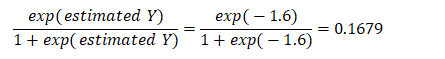
Such a person has a 16.79% chance of defaulting on the new debt. Using this probability of default, you can then use the Credit Analysis – Credit Premium model to determine the additional credit spread to charge this person given this default level and the customized cash flows anticipated from this debt holder.
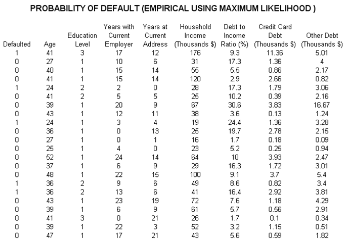
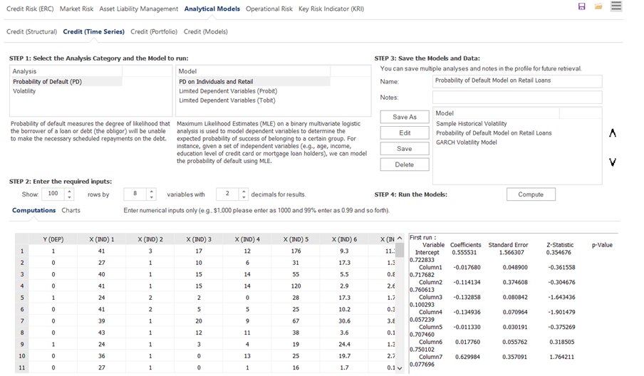
Figure 3.2: Empirical Analysis of Probability of Default