For data that exhibit a trend but no seasonality, the double moving average and double exponential smoothing methods work rather well.
Double Moving Average
The double moving average method will smooth out past data by performing a moving average on a subset of data that represents a moving average of an original set of data. That is, a second moving average is performed on the first moving average. The second moving average application captures the trending effect of the data. Figures 12.9 and 12.10 illustrate the computation involved. The example shown is a 3-month double moving average and the forecast value obtained in period 40 is calculated using the following:
![]()
where the forecast value is twice the amount of the first moving average (MA1) at time t, less the second moving average estimate (MA2) plus the difference between the two moving averages multiplied by a correction factor (two divided into the number of months in the moving average, m, less one).
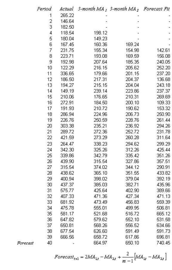
Figure 12.9: Double Moving Average (3 Months)
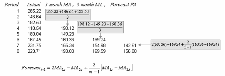
Figure 12.10: Calculating Double Moving Average
Double Exponential Smoothing
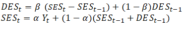
The second approach to use when the data exhibit a trend but no seasonality is the double exponential-smoothing method. Double exponential smoothing involves applying single exponential smoothing twice, once to the original data and then a second time to the resulting single exponential-smoothing data. An alpha (α) weighting parameter is used on the first or single exponential smoothing (SES) while a beta (β) weighting parameter is used on the second or double exponential smoothing (DES). This approach is useful when the historical data series is not stationary. Figure 12.11 illustrates the double exponential-smoothing model, while Figure 12.12 shows Excel’s Solver add-in dialog box used to find the optimal alpha and beta parameters that minimize the forecast errors. Risk Simulator’s time-series forecast module takes care of finding the optimal alpha level automatically as well as allow the integration of risk simulation parameters, but we show the manual approach here using Solver as an illustrative example. Figure 12.13 shows the computational details. The forecast is calculated using the following:
The double exponential smoothing algorithm starts with a time series of historical data (denoted as the Actual column in Figure 12.11) in chronological order. The example historical data shows 39 periods, and we need to forecast 4 periods into the future (periods 40–43). The first step is to create the SES and DES columns using the two equations shown above. To get started and as placeholders, set α = 0.1593 and β = 0.3913 so that these two columns can be computed. See Figure 12.13 for more detailed calculations of these two columns.
Then, create the last column called Forecast Fit (Figure 12.11). This last column is computed using the equation:
![]()
Note that in the equation above, N = 1 for all in-sample forecasts (i.e., for periods 3–39). It is typically standard to leave out the first two periods’ forecast fit values in a double exponential smoothing method to avoid any zero outlier issues for the beginning periods. For instance, period 3’s forecast fit is 246.33 + 1 × (–7.40) = 238.93, and period 4’s forecast fit is 229.94 + 1 × (–10.93) = 219.01, and so forth. Notice the multiplier is always set to 1. Conversely, when we perform out-of-sample forecasts, the multiplier N ≥ 1. For instance, the first forecast (period 40) value is computed as 690.24 + 1 × 27.91 = 718.14 (rounded) and second forecast (period 41) value is 690.24 + 2 × 27.91 = 746.05 (rounded), and so forth, with each successive future forecast increasing the index N by 1.
The reason for the index N to increment by 1 in each out-of-sample forecast is because the SES and DES columns can only be computed until the last period of the Actual data. In other words, there are 39 actual historical data points, which means we can only compute 39 rows of SES and DES. In turn, only 39 periods of Forecast Fit can be computed as well. To extrapolate and forecast beyond this set of historical data, the incremental index N is required.
Finally, to get the best-fitting α and β parameters, optimization is used to minimize the RMSE errors (Figure 12.12) and the optimized values are found to be α = 0.1593 and β = 0.3919. Note that both parameters must be between 0 and 1, inclusive. Figure 12.11 shows the calculations and results of the entire double exponential-smoothing algorithm.
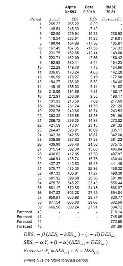
Figure 12.11: Double Exponential Smoothing
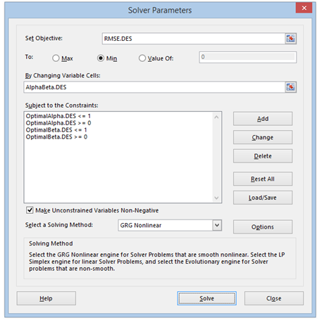
Figure 12.12: Optimizing Parameters in Double Exponential Smoothing
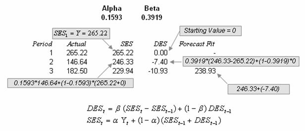
Figure 12.13: Calculating Double Exponential Smoothing