In the world of project management, there are essentially two major sources of risks: schedule risk and cost risk. In other words, will the project be on time and under budget, or will there be a schedule crash and budget overrun, and, if so, how bad can they be? To illustrate how quantitative risk management can be applied to project management, we use ROV PEAT to model these two sources of risks.
To follow along, start the PEAT software, select the Project Management––Dynamic Cost and Schedule Risk module, and Load Example. We begin by illustrating a simple linear path project in the Simple Linear Path 1 tab (Figure TN.31). Note that users can click on the Projects menu to add additional projects, or delete and rename existing projects. The example loaded has 5 sample predefined projects. In this simple linear path project, there are 11 sample tasks in this project and each task is linked to its subsequent tasks linearly (i.e., Task 2 can only start after Task 1 is done, and so forth). For each project, a user has a set of controls and inputs:
- Sequential Path versus Complex Network Path. The first example illustrated uses the sequential path, which means there is a simple linear progression of tasks. In the next example, we will explore the complex network path where tasks can be executed linearly, simultaneously, and recombined at any point in time.
- Fixed Costs. The fixed costs and their ranges suitable for risk simulation (minimum, most likely, maximum) are required inputs. These fixed costs are costs that will be incurred regardless if there is an overrun in the schedule (the project can be completed early or late, but the fixed costs will be the same regardless).
- Time Schedule. Period-specific time schedule (minimum, most likely, maximum) in days, weeks, or months. Users will first select the periodicity(e.g., days, weeks, months, or unitless) from the droplist and enter the projected time schedule per task. This schedule will be used in conjunction with the variable cost elements (see next bullet item), and will only be available if Include Schedule-Based Cost Analysis is checked.
- Variable Cost. This is the variable cost that is incurred based on the time schedule for each task. This variable cost is per period and will be multiplied by the number of periods to obtain the total variable cost for each task. The sum of all fixed costs and variable costs for all tasks will of course be the total cost for the project (denoted as Project Total Cost ).
- Overrun Assumption. This is a percent budget buffer or cushion to include in each task. This column is only available and used if the Include Budget Overruns and Buffers checkbox is selected.
- Probability of Success. This allows users to enter the probability of each task being successful. If a task fails, then all subsequent tasks will be canceled, and the costs will not be incurred, as the project stops and is abandoned. This column is available and will be used in the risk simulation only if the Include Probabilities of Success checkbox is selected.
- Run. The run button will perform the relevant computations based on the settings and inputs, and also run risk simulations if the Perform Risk Simulation checkbox is selected (as well as the requisite simulation settings such as distribution type, number of trials, and seed value settings are entered appropriately). This will run the current project’s model. If multiple projects need to be run, you can first proceed to the Portfolio Analysis tab and click on the Run All Projects button instead.
To see which of these input assumptions drive total cost and schedule the most, a tornado analysis can be executed (Figure TN.32). The model can then be risk simulated and the results show probability distributions of cost and schedule (Figure TN.33). For instance, the sample results show that for Project 1, there is a 95% probability that the project can be completed at a cost of $398,594. The originally expected median or the most likely value was $377,408 (Figure TN.31). With simulation, it shows that to be 95% sure that there are sufficient funds to complete the project, an additional buffer of $21,186 is warranted.
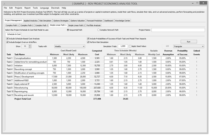
Figure TN.31: Simple Linear Path Project Management with Cost and Schedule Risk
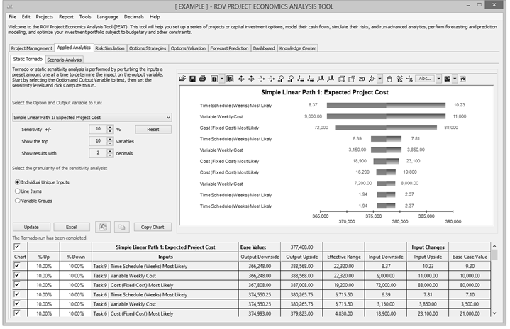
Figure TN.32: Simple Linear Path Tornado Analysis
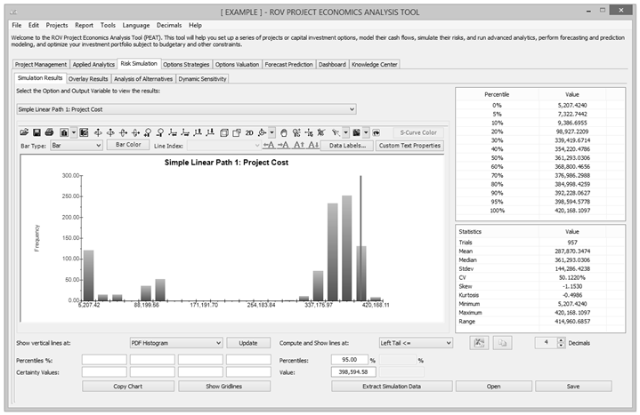
Figure TN.33: Monte Carlo Risk Simulated Results for Risky Cost and Schedule Values
In complex projects where there are nonlinearly bifurcating and recombining paths (Figure TN.34), the cost and schedule risk modeling is more difficult to model and compute. For instance, in the Complex Path 1 tab, we can see that after Task 1, future tasks can be run in parallel (Tasks 2, 3, and 4). Then, Tasks 3 and 4 recombine into Task 8. Such complex path models can be created by the user simply by adding tasks and combining them in the visual map as shown. The software will automatically create the analytical financial model when Create Model is clicked. That is, you will be taken to the Schedule & Cost tab and the same setup as shown previously is now available for data entry for this complex model (Figure TN.35). The complex mathematical connections will automatically be created behind the scenes to run the calculations so that the user will only need to perform very simple tasks of drawing the complex network path connections. Below are some tips on getting started:
- Start by adding a new project from the Projects Then, click on the Complex Network Path radio selection to access the Network Diagram tab.
- Use the icons to assist in drawing your network path. Hover your mouse over the icons to see their descriptions. You can start by clicking on the third icon to Create a Task, and then click anywhere in the drawing canvas to insert said task.
- With an existing task clicked on and selected, click on the fourth icon to Add a Subtask. This will automatically create the adjoining next task and next task number. You then need to move this newly inserted task to its new position. Continue with this process as required to create your network diagram. You can create multiple subtasks off a single existing task if simultaneous implementations occur.
- You can also recombine different tasks by clicking on one task, then holding down the Ctrl key, click on the second task you wish to join. Then click on the fifth icon to Link Tasks to join then. Similarly, you can click on the sixth icon to Delete Link between any two tasks.
- When the network diagram is complete, click on Create Model to generate the computational algorithms where you can then enter the requisite data in the Schedule & Cost tab as described previously.
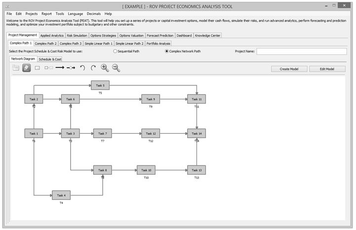
Figure TN.34: Complex Path Project Management
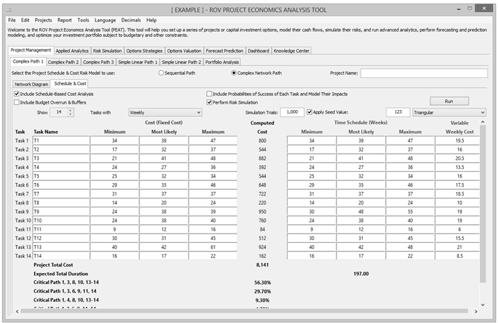
Figure TN.35: Complex Project Simulated Cost and Duration Model with Critical Path
After running the model, the complex path map shows the highlighted critical path (Figure TN.36) of the project, that is, the path that has the highest potential for bottlenecks and delays in completing the project on time. The exact path specifications and probabilities of being on the critical path are seen in Figure TN.35 (e.g., there is a 56.30% probability that the critical path will be along Tasks 1, 3, 8, 10, 13, 14).
If there are multiple projects or potential project path implementations, the portfolio view (Figure TN.37) compares all projects and implementation paths for the user to make a better and more informed risk-based decision. The simulated distributions can also be overlaid (Figure TN.38) for comparison.
Figure TN.37 allows users to see all projects that were modeled at a glance. Each project modeled can actually be different projects or the same project modeled under different assumptions and implementation options (i.e., different ways of executing the project), to see which project or implementation option path makes more sense in terms of cost and schedule risks. The Analysis of Alternatives radio selected allows users to see each project as standalone (as compared to Incremental Analysis where one of the projects is selected as the base case and all other projects’ results show their differences from the base case), in terms of cost and schedule: single-point estimate values, simulated averages, the probabilities each of the projects will have a cost or schedule overrun, and the 90th percentile value of cost and schedule. Of course, a more detailed analysis can be obtained from the Risk Simulation | Simulation Results tab, where users can view all the simulation statistics and select any confidence and percentile values to show. This Portfolio Analysis tab also charts the simulated cost and schedule values using bubble and bar charts for a visual representation of the key results.
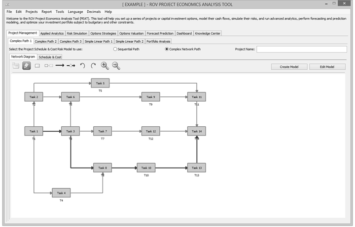
Figure TN.36: Complex Project Critical Path
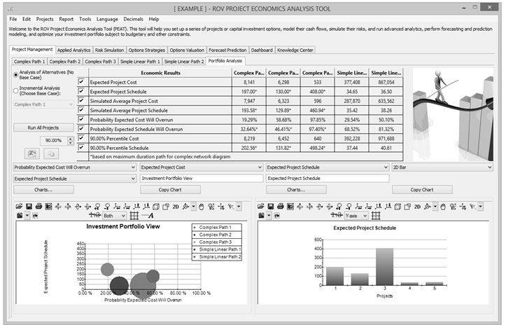
Figure TN.37: Portfolio View of Multiple Projects at Once
The Overlay chart in Figure TN.38 shows multiple projects’ simulated costs or schedules overlaid on top of one another to see their relative spreads, location, and skew of the results. We clearly see that the project whose distribution lies to the right has a much higher cost to complete than the left, with the project on the right also having a slightly higher level of uncertainty in terms of cost spreads. Refer to the chapter on Test Driving Risk Simulator and Technical Note 1 for more details on interpreting these PDF and CDF charts, as well as how to make better and more informed decisions using their results.
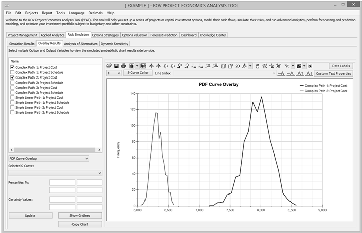
Figure TN.38: Overlay Charts of Multiple Projects’ Cost or Schedule