The two-sample equal variance t-test, as its name suggests, compares two sample datasets against each other to determine if there is a statistically significant difference between their population means (μ). In other words, the test can identify if a certain event or experiment has an effect. This t-test assumes that the unknown population standard deviations (σ) of both samples are roughly equal, and the populations are roughly normally distributed. The t-distribution is appropriate here as the true standard deviations of the populations are unknown, and when smaller sample sizes are available (typically < 30). This test is also known as the pooled-variances t-test because it takes the standard deviations of both samples and pools them into a single parameter in the model.
The hypotheses tested are typically:
H0: μ1 = μ2 that is, the two samples’ means are statistically similar
Ha: μ1 ≠ μ2 that is, the two samples’ means are statistically significantly different
As a reminder, the null hypothesis (H0) generally has the equivalence sign (i.e., =, ≥, ≤), whereas the alternate hypothesis (Ha) has its complement (i.e., ≠, <, >). The sign of the alternate hypothesis points to whether the test is a two-tailed test (≠) or a one-tailed test (right tail is denoted with >, whereas a left tail test uses <).
To get started, two datasets with several data points (with n1 and n2 sample sizes) are put side by side (see Figure 9.2). Then, their respective sample averages (x̅1 and x̅2) and sample standard deviations (s1 and s2) are computed. The t-statistic is then calculated using the formula below and compared against the critical t-values. In most situations, the p-value of this calculated t-statistic is calculated and compared against some predefined level of significance (i.e., the standard a significance levels of 0.10, 0.05, and 0.01 will be assumed throughout these examples) using the t-distribution with a certain degree of freedom (df). If the p-value is below these α significance levels, we reject the null hypothesis and accept the alternate hypothesis (Figure 9.1).
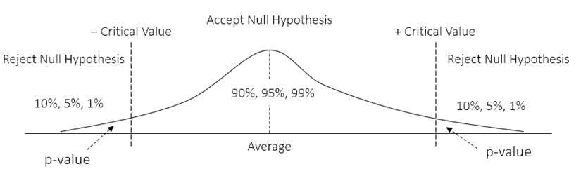
Figure 9.1: Visual Representation of Acceptance/Rejection Regions
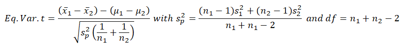
The formal specification of the two-sample equal variance test is:
As seen in Figure 9.2, the model was run in Microsoft Excel’s Data Analysis Toolkit. The t-statistic was computed as –1.2273, and the two-tail p-value is 0.2355, corresponding to a two-tailed critical t-value of ±2.1009. As explained in previous chapters, if the calculated t-statistic exceeds these critical t-values, we reject the null hypothesis, otherwise, we will fail to reject the null and summarily accept the alternate hypothesis. An alternate, and perhaps a simpler, approach is to compare the computed p-value against the a significance level. If the p-value is ≤ α, then we reject the null hypothesis.
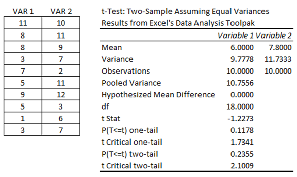
Figure 9.2: Two-Sample Equal Variance T-Test
Based on the calculations above, the p-value exceeds the standard 0.10, 0.05, 0.01 thresholds, which means we fail to reject the null hypothesis and conclude that the two sample datasets are statistically not different from one another and that whatever experiment or treatment was applied was ineffective. Please note that in this example, we test H0: μ1 = μ2 which means that in the equation, we set μ1 – μ2 = 0. This also means we need to set the hypothesized mean to 0 in BizStats (Figure 9.4).
The analysis can be done manually (Figure 9.3 shows the manual computations performed in Excel and you can see the corresponding cell equations) using the model specification provided above, or by using the ROV BizStats software (Figure 9.4).
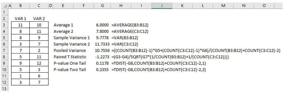
Figure 9.3: Manual Computations
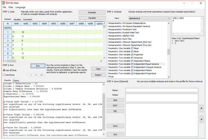
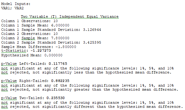
Figure 9.4: ROV BizStats Calculations
To use the ROV BizStats tool, make sure that ROV Risk Simulator is installed on your computer. Then, start Excel, click on the Risk Simulator menu and select ROV BizStats from the icon ribbon. You will see a user interface similar to Figure 9.4. In Step 1’s data grid, you can now manually enter the two datasets or copy and paste from another source such as Microsoft Excel or another database or text file. Next, select the relevant analysis in Step 2. In this specific example, the Parametric Two Variable (T) with Independent and Equal Variances should be selected. When this item is selected, you will see the sample data requirements (e.g., Data = 2 Variables, Hypothesized Mean, and examples VAR1, VAR2). Next, either manually type in VAR1; VAR2 separated by a semicolon, then hit enter and type 0 into the input box in Step 2 for the hypothesized difference, or simply double click the variable header (e.g., VAR1 and then VAR2) to add these variables automatically. Next, just hit Run to perform the calculations. You can see that the results confirm both the manual computations and Excel Data Analysis Toolkit results (e.g., t-statistic is –1.2273 and p-value is 0.2355).