The model used is Value at Risk – Portfolio Operational and Capital Adequacy and is accessible through Modeling Toolkit | Value at Risk | Portfolio Operational and Capital Adequacy. This model shows how operational risk and credit risk parameters are fitted to statistical distributions and their resulting distributions are modeled in a portfolio of liabilities to determine the Value at Risk (e.g., 99.50th percentile certainty) for the capital requirement under Basel III/IV and III requirements. It is assumed that the historical data of the operational risk impacts (Historical Data worksheet) are obtained through econometric modeling of the Key Risk Indicators.
The Distributional Fitting Report worksheet is a result of running a distributional fitting routine in Risk Simulator to obtain the appropriate distribution for the operational risk parameter. Using the resulting distributional parameters, we model each liability’s capital requirements within an entire portfolio. Correlations can also be inputted if required, between pairs of liabilities or business units. The resulting Monte Carlo simulation results show the Value at Risk or VaR capital requirements.
Note that an appropriate empirically based historical VaR cannot be obtained if distributional fitting and risk-based simulations were not first run. Only by running simulations will the VaR be obtained. To perform distributional fitting, follow the steps below:
-
- In the Historical Data worksheet (Figure 2.11), select the data area (cells C5:L104) and click on Risk Simulator | Analytical Tools | Distributional Fitting (Single Variable).
- Browse through the fitted distributions and select the best-fitting distribution (in this case, the exponential distribution with a particularly high p-value fit, as shown in Figure 2.12), and click OK.
- You may now set the assumptions on the Operational Risk Factors with the exponential distribution (fitted results show Lambda = 1) in the Credit Risk worksheet. Note that the assumptions have already been set for you in advance. You may set them by going to cell F27 and clicking on Risk Simulator | Set Input Assumption, selecting Exponential distribution and entering 1 for the Lambda value, and clicking OK. Continue this process for the remaining cells in column F or simply perform a Risk Simulator Copy and Risk Simulator Paste on the remaining cells:
- Note that since the cells in column F have assumptions set, you will first have to clear them if you wish to reset and copy/paste parameters. You can do so by first selecting cells F28:F126 and clicking on the Remove Parameter icon or select Risk Simulator | Remove Parameter.
- Then select cell F27, click on the Risk Simulator Copy icon or select Risk Simulator | Copy Parameter, and then select cells F28:F126 and click on the Risk Simulator Paste icon or select Risk Simulator | Paste Parameter.
- Next, additional assumptions can be set such as the probability of default using the Bernoulli distribution (column H) and Loss Given Default (column J). Repeat the procedure in Step 3 if you wish to reset the assumptions.
- Run the simulation by clicking on the Run icon or clicking on Risk Simulator | Run Simulation.
- Obtain the Value at Risk by going to the forecast chart once the simulation is done running and selecting Left-Tail and typing in 50. Hit Tab on the keyboard to enter the confidence value and obtain the VaR of $25,959 (Figure 2.13).
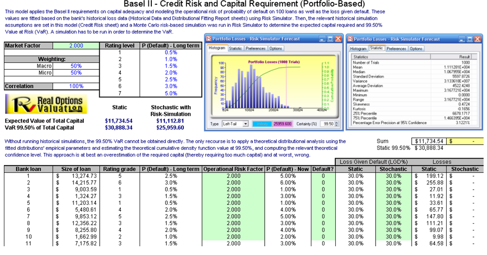
Figure 2.11: Sample Historical Bank Loans
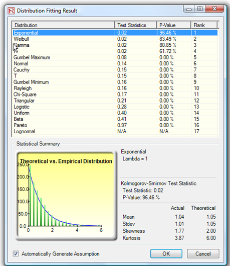
Figure 2.12: Data Fitting Results
Another example of VaR computation is shown next, where the model Value at Risk – Right Tail Capital Requirements is used and available through Modeling Toolkit | Value at Risk | Right Tail Capital Requirements. This model shows the capital requirements per Basel III/IV and III requirements (99.95th percentile capital adequacy based on a specific holding period’s Value at Risk). Without running risk-based historical and Monte Carlo simulation using Risk Simulator, the required capital is $37.01M (Figure 2.14) as compared to only $14.00M required using a correlated simulation (Figure 2.15). This is due to the cross-correlations between assets and business lines and can only be modeled using Risk Simulator. This lower VaR is preferred as banks can now be required to hold less capital and can reinvest the remaining capital in various profitable ventures, thereby generating higher profits.
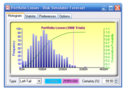
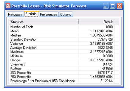
Figure 2.13: Simulated Forecast Results and the 99.50% Value at Risk Value
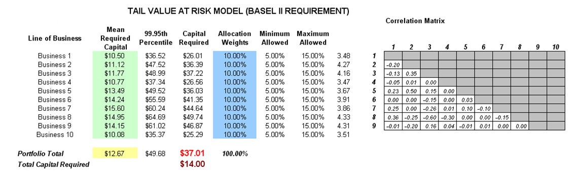
Figure 2.14: Right-tail VaR Model
-
-
- To run the model, click on Risk Simulator | Run Simulation (if you had other models open, make sure you first click on Risk Simulator | Change Simulation | Profile, and select the Tail VaR profile before starting).
- When the simulation is complete, select Left-Tail in the forecast chart and enter in 95 in the Certainty box, and hit TAB on the keyboard to obtain the value of $14.00M Value at Risk for this correlated simulation.
- Note that the assumptions have already been set for you in advance in the model in cells C6:C15. However, you may set them again by going to cell C6 and clicking on Risk Simulator | Set Input Assumption, selecting your distribution of choice or using the default Normal Distribution or performing a distributional fitting on historical data, and click OK. Continue this process for the remaining cells in column C. You may also decide to first Remove Parameters of these cells in column C and setting your own distributions. Further, correlations can be set manually when assumptions are set (Figure 2.16) or by going to Analytical Tools | Edit Correlations (Figure 2.17) after all the assumptions are set.
-
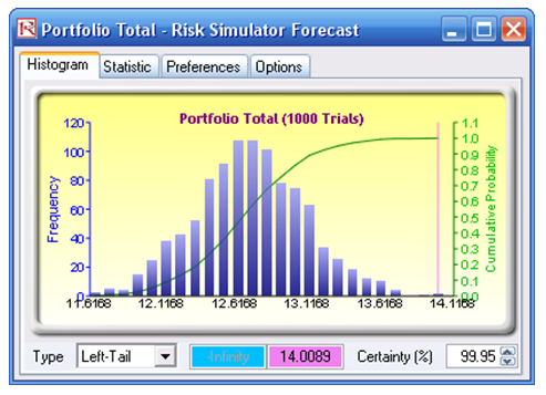
Figure 2.15: Simulated Results of the Portfolio VaR
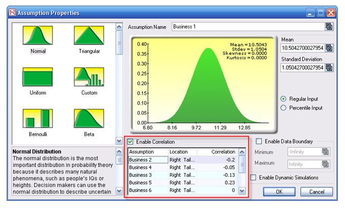
Figure 2.16: Setting Correlations One at a Time
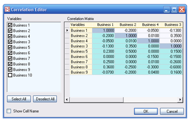
Figure 2.17: Setting Correlations Using the Correlation Matrix Routine
If risk simulation was not run, the VaR or economic capital required would have been $37M, as opposed to only $14M. And all cross-correlations between business lines have been modeled, as are stress and scenario tests, as well as thousands and thousands of possible iterations having been run. Individual risks are now aggregated into a cumulative portfolio level VaR.