The example file is Probability of Default – Empirical and can be accessed through Modeling Toolkit | Prob of Default | Empirical (Individuals). To run the analysis, select the dataset (include the headers) and make sure that the data have the same length for all variables, without any missing or invalid data points. Then, using Risk Simulator, click on Risk Simulator | Forecasting | Maximum Likelihood Models. A sample set of results is provided in the MLE worksheet, complete with detailed instructions on how to compute the expected probability of default of an individual.
The MLE approach applies a modified binary multivariate logistic analysis to model dependent variables to determine the expected probability of success of belonging to a certain group. For instance, given a set of independent variables (e.g., age, income, education level of credit card or mortgage loan holders), we can model the probability of default using MLE. A typical regression model is invalid because the errors are heteroskedastic and non-normal, and the resulting estimated probability forecast will sometimes be above 1 or below 0. MLE analysis handles these problems using an iterative optimization routine. The computed results show the coefficients of the estimated MLE intercept and slopes.¹
The coefficients estimated are actually the logarithmic odds ratios and cannot be interpreted directly as probabilities. A quick but simple computation is first required. The approach is simple. To estimate the probability of success of belonging to a certain group (e.g., predicting if a debt holder will default given the amount of debt he or she holds), simply compute the estimated Y value using the MLE coefficients. Figure 2.6 illustrates an individual with 8 years at a current employer and current address, a low 3% debt to income ratio, and $2,000 in credit card debt has a log-odds ratio of –3.1549. Then, the inverse antilog of the odds ratio is obtained by computing:
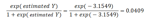
So, such a person has a 4.09% chance of defaulting on the new debt. Using this probability of default, you can then use the Credit Analysis – Credit Premium model to determine the additional credit spread to charge this person given this default level and the customized cash flows anticipated from this debt holder.
¹For instance, the coefficients are estimates of the true population b values in the following equation: Y = b 0 + β1X1 + β2X2 + … + βnXn. The standard error measures how accurate the predicted coefficients are, and the Z-statistics are the ratios of each predicted coefficient to its standard error. The Z-statistic is used in hypothesis testing, where we set the null hypothesis (Ho) such that the real mean of the coefficient is equal to zero, and the alternate hypothesis (Ha) such that the real mean of the coefficient is not equal to zero. The Z-test is very important as it calculates if each of the coefficients is statistically significant in the presence of the other regressors. This means that the Z-test statistically verifies whether a regressor or independent variable should remain in the model or should be dropped. That is, the smaller the p-value, the more significant the coefficient. The usual significant levels for the p-value are 0.01, 0.05, and 0.10, corresponding to the 99%, 95%, and 90% confidence levels.
![]()
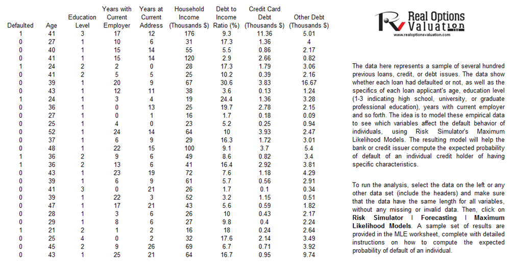
Figure 2.5: Empirical Analysis of Probability of Default
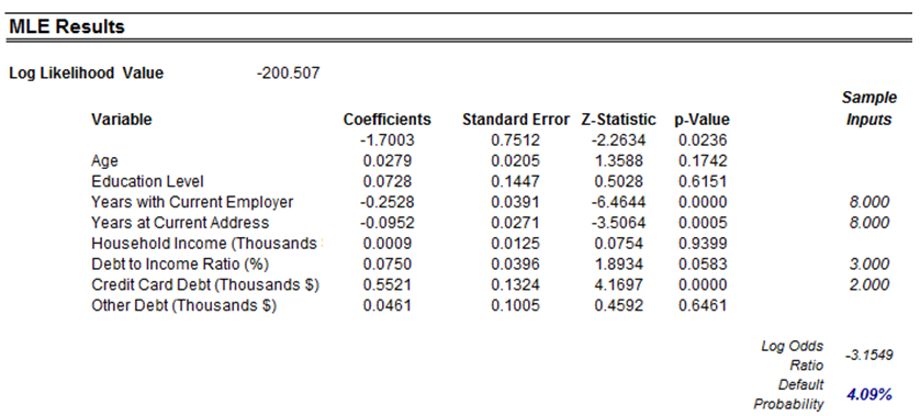
Figure 2.6: MLE Results